COVID19: How many are missing?
What does it take to estimate the number of undetected cases?
Jeremy, 12 June 2020
The code used for making the plots and the regressions can be found here
In the COVID-19 pandemic, one interesting quantity one might want to estimate is the proportion \(p_{nd}\) of infected people that are not detected by the tests (on a given date or period of time). We can, for that, estimate the proportion of infected people \(p_d:= 1-p_{nd}\) that have been detected (the subscripts \(d\) and \(nd\) respectively stand for detected and not detected). There are many reasons why not all infectious persons are detected: For example, many people might only have mild symptoms, and therefore do not try to get tested. Another reason is that we simply do not have enough tests to test all the infectious people, and therefore we need to prioritize by choosing who gets to be tested and who does not. In the first case, and if the tests were cheap and abundant, then a relatively easy solution exists to estimate the proportion of undetected infectious people: We can pick a random sample of the population that we get tested. From this, we can measure the proportion of infectious people within the sample, and by the law of large-numbers this proportion should equal the proportion of infectious people in the whole population (up to statistical fluctuations related to the size of the sample). Knowing this and the number of detected infectious people we can deduce the proportion of undetected infectious people.
However, when the number of test per day, or per week, is limited one cannot necessarily test a sufficiently large random sample of the population. Moreover, if today we want to estimate what was \(p_{nd}\) at the beginning of the pandemic, i.e. several weeks ago, one needs to have access to the results of tests that would have been performed on a random sample of the population at the time for which we wish to make our estimation. If no test has been performed on such a random sample, the technique fails by lack of available data, and we need to use other data and ways of estimating \(p_{nd}\).
This is what the authors of [LPJ*] have done. In this post I will explain the principles underlying such an estimation method for \(p_{d}\) (or equivalently \(p_{nd}\)) through an analogue but simpler analysis using data about the total number of confirmed COVID-19 cases.
I will try as much as possible to draw parallels between my simplified approach and the work done in [LPJ*].
The Data
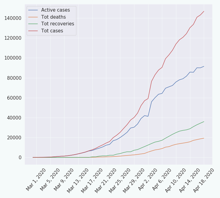
I have taken the data from worldometer.com (for France) from which I have made a csv file. It represents the evolution of the following quantities through time:
| 1. the daily new cases | 2. the total cases |
| 3. the daily new recoveries | 4. the total recoveries |
| 5. the daily new deaths | 6. the total deaths |
| 7. the active cases. |
The Models
The model I have used
In the following I will modtly describe my model in a graphical way. If you want to have a bit more mathematical details about my model, you can read the model section of this document.
Some explanations on the traditional SIRD model
In order to analyse the data of the COVID-19 I will use a variation of the SIRD model. SIRD stands for Susceptible Infectious Recovered Dead. It is a simple model for epidemiology that works as follows: The studied population, comprised of N individuals, is divided into four categories: susceptible (S), infectious (I), recovered (R), dead (D). For each of these categories the model describes the evolution of the number of people belonging to these categories as a function of time. To do so the model uses the following system of four differential equations,
\[\begin{cases} \frac{dS}{dt}= -\beta I \frac{S}{N}\\ \frac{dI}{dt}= \beta I \frac{S}{N} - \gamma I - \mu I\\ \frac{dR}{dt}= \gamma I\\ \frac{dD}{dt}= \mu I\\ \end{cases}\]The first line intuitively reads as follows: during a small amount of time \(dt\) the susceptible population \(S\) (i.e. the not infected part population but that is still susceptible to get infected) varies by an amount \(dS = -\beta I \frac{S}{N} dt\). This means that if at time \(t_0\) there are \(S(t_0)\) susceptible people, at time \(t_0+dt\) there are \(S(t_0+dt)=S(t_0)+dS = S(t_0)-\beta I \frac{S}{N} dt\). Since \(dS\) is negative, the population \(S\) decreases with time, i.e. there are less and less not-infected people through time. The quantity \(|dS|\) represents the number of new cases of COVID-19 that have occurred during the duration \(dt\).
Let us see why we have \(dS = -\beta I \frac{S}{N} dt\). Let us say that each infectious person infects on average a fraction \(f_{\rm inf}\) of the susceptible person they meet, and that on average they meet \(\kappa \times dt\) persons during the time \(dt\). Importantly, not all the people they meet are susceptible. If we assume that people meet each other in a sufficiently random way, then there should be a fraction \(\frac{S}{N}\) (where \(N\) is the total size of the studied population) of the people the infectious person has met that are susceptible. In other words, each of the infectious people meets on average \(\kappa \times dt \times \frac{S}{N}\) susceptible persons and infects a fraction \(f_{\rm inf}\) of them, i.e. they infect on average \(f_{\rm inf} \times \kappa \times dt \times \frac{S}{N}\) people. Since there are \(I\) infectious people, each of them infecting on average \(f_{\rm inf} \times \kappa \times dt \times \frac{S}{N}\) people, there are in total \(|dS| = I\times f_{\rm inf} \times \kappa \times dt \times \frac{S}{N}\) new infections during the time \(dt\). By defining \(\beta := f_{\rm inf} \times \kappa\) we get the desired result: \(dS = -\beta I \frac{S}{N} dt\) (remember that \(dS\) must be negative since \(S\) must decrease). The parameter \(\beta\) is the rate a which each of the infectious people infects other people.
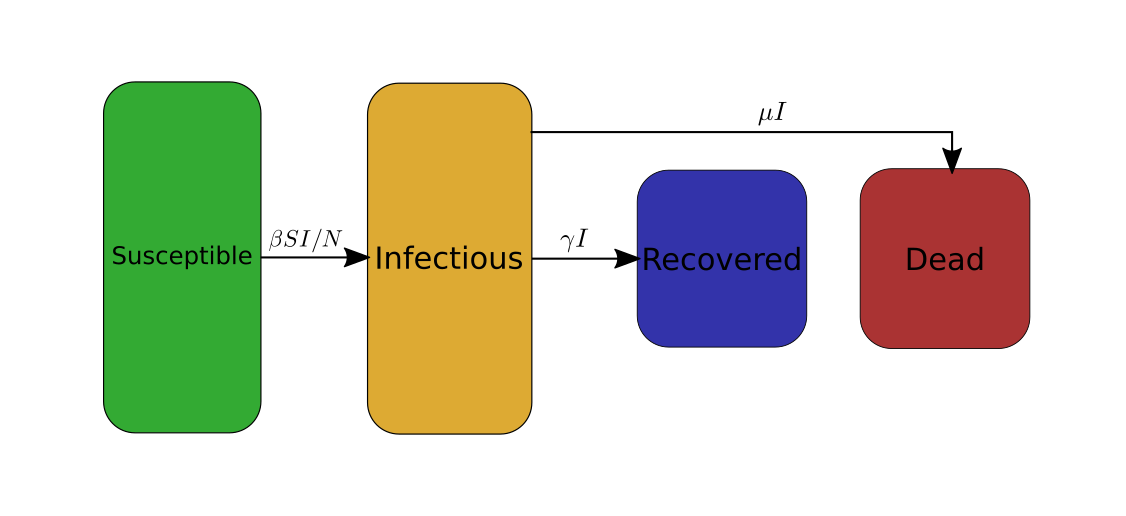
Similarly, the three other equations respectively describe how the numbers \(I\) of infectious people, \(R\) of recovered people, and \(D\) of dead people evolve through time. The parameter \(\gamma\) is the rate at which infectious people recover from the COVID-19, and \(\mu\) is the rate at which they die from COVID-19.
To avoid the use of equations, I will, from now on, graphically represent the SIRD model as follows.
Modifications
First ingredient: split categories
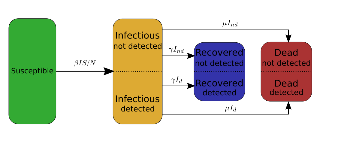
In my case I need to make the distinction between the infectious people that have been tested and detected, and the infectious people that have not been detected. Therefore, I will split the infectious category into two subcategories \(I_d\) and \(I_{nd}\), and similarly split the recovered category into two subcategories \(R_d\) and \(R_{nd}\), and the deaths category into \(D_d\) and \(D_{nd}\). The SIRD model then becomes,
Second ingredient: Aggregate several categories into one of particular interest (\(T_d\))
From the above model we can extract one extra category of particular interest. This particular category is the category of the all the cases of COVID-19. As for other categories, part of these cases remains undetected. Therefore, I will use the quantity \(T_d\), \(T_{nd}\), and \(T:= T_d+T_nd\) to denote the total number of detected, undetected, and overall cases respectively. By definition \(T_d:=I_d+R_d+D_d\), and \(T_{nd} := I_{nd} + R_{nd} + D_{nd}\). \(T_d\) is of particular interest for two reasons:
- \(T_d\) is a quantity we can actually observe as opposed to \(T_{nd}\) or \(T\).
- From the equations describing the model presented in the above figure, we can deduce that \(T_d = p_d T\). An interesting consequence of this is that the rate at which \(T_d\) evolves is the same as the rate at which \(T\) evolves, which turns out to be \(\beta\). In other words, the evolution of \(T_d\), which only concerns the detected people, actually gives us information about the evolution of the whole category \(T\) of the people that have been infected at some point, whether they have been detected or not.

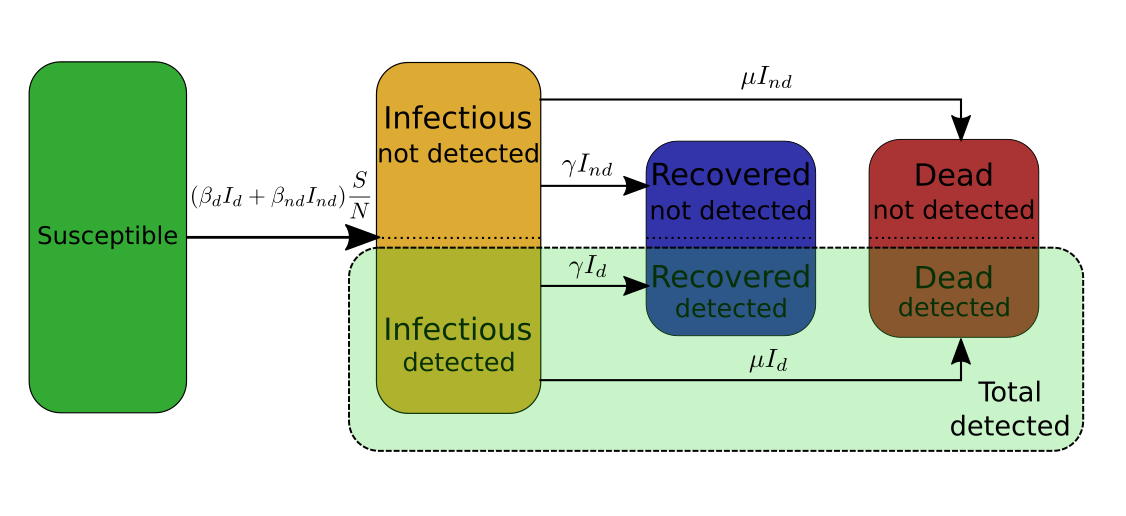
Last ingredient: split \(\beta\)
Finally, the last ingredient for the model is to split \(\beta\) into \(\beta_d\) for the population \(I_d\), and \(\beta_{nd}\) for the population \(I_{nd}\) so that \(\beta I = \beta_d I_d + \beta_{nd} I_{nd}\). From the equations of the SIRD model one can deduce that \(I_d=p_d I\) and \(I_{nd} = (1-p_d) I\), which implies that \(\beta=p_d \beta_d +(1-p_d) \beta_{nd}\).
The model used in [LPJ*]
In [LPJ*] the authors use a variation of the SIERD model. The SIERD model has one more category than the SIRD model, namely it considers the category exposed (E) of exposed people, i.e. of people that have been contaminated by the virus but that are not yet infectious. The model used by the authors is different in three ways from the traditional SIERD model:
- The model does not consider only one population split in 5 categories. It actually considers the population of several cities, and split the population of each of these cities into the five categories of the SIERD. Each city’s population is modelled by a system of equations similar to the one for the SIRD model above. Furthermore, their model allows for population exchanges between the cities, which couples each city’s system of equations with each other.
- The authors consider a stochastic version of the SIERD model, meaning that they introduce some randomness in the model. This allows to more carefully account for statistical fluctuations and uncertainties.
- For every city, the Infectious category is split into two subcategories: detected and undetected.
Using the model
Some intuition
In this section we will assume that \(\beta\) can be extracted from the data so that it is considered as a known parameter.
Remember that \(\beta = p_d \beta_d + (1-p_d) \beta_{nd}\). Let us say that at the beginning of the pandemic no measures are taken against it, and therefore both the detected cases and the undetected cases can contaminate new people, i.e. \(\beta_d, \beta_{nd} >0\).
What would happen if we suddenly decided to strictly quarantine the detected cases, so that they cannot
contaminate anyone anymore (i.e. \(\beta_d = 0\))?
Assuming that this is the only preventive measure taken against the pandemic (in particular no measures are taken
for the undetected cases: \(\beta_{nd}\) does not change), the value of \(\beta\) would actually change
to a smaller value. The extent by which the value of \(\beta\) diminishes depends on \(p_d\). Indeed, since \(\beta = p_d
\beta_d + (1-p_d) \beta_{nd}\), setting \(\beta_d\) to \(0\) has a bigger effect on the value of \(\beta\) when \(p_d\) is
large than when \(p_d\) is small. This means that if one estimate the value of \(\beta\) before the quarantine measure and
compares it with its value before the quarantine measure, one will get some information about \(p_d\).
Preliminary conclusion 1: The observable repercussions of the difference of treatment between the detected and not detected subcategories allow to extract some information about \(p_d\). This is a key point of [LPJ*]. In their model, the detected infectious people cannot travel from city to city, while the other people can (which includes the undetected infectious people). The consequence is that the speed at which the COVID-19 spreads to other cities highly depends on the parameter \(p_d\):
- If \(p_d\) is very high, i.e. most of the infectious people are detected, then very few infectious people can travel, and the COVID-19 should spread slowly to other cities.
- On the contrary, if \(p_d\) is small, then many infectious people can travel, and the COVID-19 should spread faster.
Key observation
Let us try to fit the model to the data we have. More precisely I will fit \(T_d\), \(D_d\), and \(R_d\) to the collected data over 50 days, and we get the following:
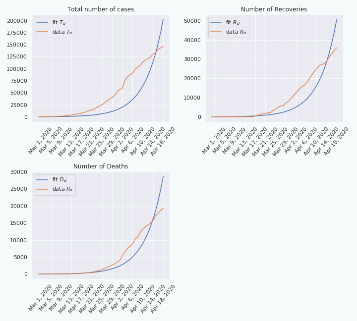
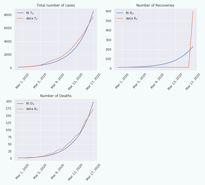
As we can see, on the top left figure, the fit is not really good. This suggests that the model cannot explain the data, at least not over a period of 50 days. Indeed, if we do the same thing over a shorter period, e.g. 18 days, the fit looks better.
From this we can make the hypothesis that the rate \(\beta\) is not constant, but is slowly changing through time. This make sense considering that preventive measures, like social distancing, have been taken to precisely decrease this rate \(\beta\). Therefore, if we fit the model at two different moments in time, we should be able to extract two different values for \(\beta\): \(\beta^{(1)}\) and \(\beta^{(2)}\). Moreover, we still have that \(\beta^{(1)} = p_d \beta_d^{(1)} +(1-p_d) \beta_{nd}^{(1)}\) and \(\beta^{(2)} = p_d \beta_d^{(2)} +(1-p_d) \beta_{nd}^{(2)}\).
In the previous section we said that a difference in the variation of the rate of the detected and not detected subcategories provoke a variation on the rate \(\beta\) that depends on the parameter \(p_d\).
To extract all the information about \(p_d\) I would need extra information about the values of \(\beta_d^{(1)}\), \(\beta_d^{(2)}\) and over the ratio \(\alpha:=\frac{\beta_{nd}^{(2)}}{\beta^{(1)}_{nd}}\). A priori they could be inferred from studies on the influence of social distancing and the increase of hygiene. However, I couldn’t find data on this, beyond the mobility data from Apple and Google, so I have let these parameters free, and you can play with them in the following interactive figure.
Remark: As you may see, the figure is quite sentive to the parameters you pick. This tells us that even if we knew the missing parameters, the prediction we would make would likely have a quite important uncertainty.
Preliminary conclusion 2: If one wants to extract the value of \(p_d\), one needs extra information, not necessarily immediately related to \(p_d\) itself, but related, or correlated to other parameters that influence the variation of \(\beta_d\) and \(\beta_{nd}\).
In [LPJ*] they also need some extra information to recover the value of \(p_d\). In their case this extra information is the daily number of people travelling between any pair of cities.
Conclusion
In this post we have seen two key ingredients on the estimation of \(p_d\):
- Include in the model a distinction between the detected cases and the undetected case (subcategories with
subscripts \(_d\) and \(_{nd}\) respectively). Include in the model something that will influence differently the
infection rate of each subcategory (\(\beta_d\) and \(\beta_{nd}\)). - Use extra information, not necessarily directly related to the disease, but that will influence the speed at which the
virus will spread.
NB: Both in my simplified model and in the model used in [LPJ*] many implicit assumptions are made. In general, they are necessary to the extraction of an estimate of the value of \(p_d\), but the estimate might be highly dependent on these assumptions. In particular, if these assumptions are not satisfied in reality, the estimation of \(p_d\) can be inaccurate. This is why a model is not reliable on its own. We need to use different model with different data, and different techniques to estimate a parameter like \(p_d\). If all these techniques converge to the same value of the parameter, then we can be confident in the accuracy of these estimations.
For example, in my model I implicitly assume that \(p_d\) is the same over the two period of time I used to estimate its value. In [LPJ*] the authors assume that \(p_d\) is the same in all the cities, and that the infection rate \(\beta\) is the same in all the cities etc.
References
[LPJ*] Li, Ruiyun, et al. “Substantial undocumented infection facilitates the rapid dissemination of novel coronavirus (SARS-CoV-2).” Science 368.6490 (2020): 489-493.
