Information Realm

Some time ago Constance Crozier made a nice animation illustrating that forecasting s-curves is hard:

I spent a humiliating amount of time learning how to make animated graphs, just to illustrate a fairly obvious point.

“Forecasting s-curves is hard”

My views on why carefully following daily figures is unlikely to provide insight.https://t.co/yrE71bUXVT

mymovie from Constance Crozier on Vimeo.

— Constance Crozier (@clcrozier) April 17, 2020

I wanted to go a small step further. Instead of trying to predict the shape of the curve in the future, what if we tried to predict the range of shapes it can have? In other words can we try to add confidence intervals to the prediction? ¹

I’ll do this in 4 different ways. In the first approach we use the fact that the data is generated by a known process, and therefore we know the probability distribution of the noise of the data. We can therefore resample the data using this noise distribution. Of course, in practice we might not always know what the noise distribution is. In this case we can use a bootstrap sampling method, which is the second approach we will see. In this two first methods we will construct confidence intervals called a “percentile intervals” by using above-mentioned the sampling methods. However, in general, percentile intervals do not always behave properly. As a consequence, we will explore another technique that is sometimes more robust called “Boot-T interval” and which uses bootstrap sampling to estimate the distribution of what is called the t-statistics. Finally, in the fourth approach we will use concentration bounds to derive the confidence interval. As we will see, the last method requires quite some assumptions and the derived interval is quite loose. The three first methods can be seen as application of the Monte Carlo method.

Table of content

1. Preliminaries
2. Percentile interval when we know the noise distribution
3. Percentile interval with bootstrap sampling
4. Boot-T interval
5. Interval based on McDiarmid inequality
6. Comparison and conclusions

Preliminaries

Model & Data

The sigmoid function we will use here as a model is:

where \(a, b, c,\) and \(d\) are the parameters of the model to be fitted.

To generate the data, we will choose \((a,b,c,d)=(1,1,6,0)\) and add Gaussian noise:

import numpy as np

def sig(x, args = (1,1,6,0)):
    #This function implements the sigmoid model described above
    a = args[0] 
    b = args[1] 
    c = args[2] 
    d = args[3]
    out = np.array(a/(1+np.exp(-b*(x-c)))+d)
    return out

#generate the data
std = 0.05
x = np.linspace(-6,6,100)
ydat=sig(x)+np.random.normal(scale=std,size=len(x))

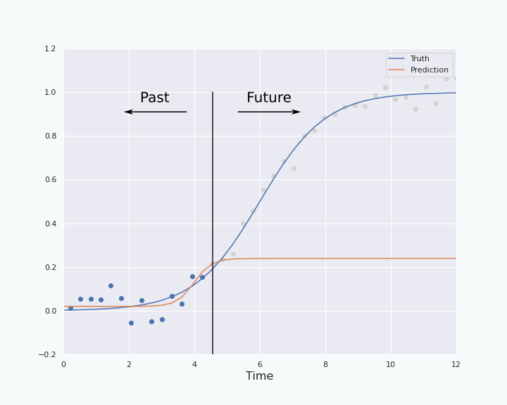
To fit the data, and therefore infer the values of \((a,b,c,d)\) from the data, we will not use the whole data but the first \(k\) points. Indeed, we want to use the first \(k\) points to predict the shape of the curve for the future points. Here is an example, created as follows,

import numpy as np
import matplotlib.pyplot as plt

#data generation
std = 0.05
x = np.linspace(0,12,100)
ydat=sig(x)+np.random.normal(scale=std,size=len(x))


#create the plot
plt.figure(figsize=(10,8))
plt.axes(xlim=(-6, 6), ylim=(-0.2, 1.2))
length = 20 #number of points considered for the fit
plt.scatter(x,ydat)
plt.plot(x, sig(x), label = "Truth")
fit_param = curve_fit(sig, x[:length], ydat[:length], [1,1,0,0]) #infer the parameter of the model by fitting the curve the k first points (k=length)
plt.plot(x,sig(x,fit_param['x']), label = "Prediction")
plt.plot([x[length],x[length]], [0,1])
plt.legend(loc = 'best')

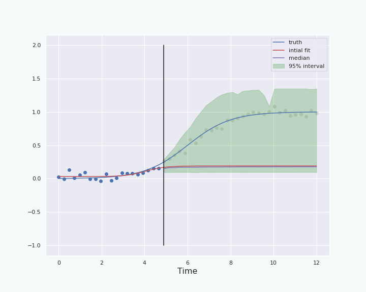
Percentile interval when we know the noise distribution

In this section we will use a percentile interval using the fact that we know the probability distribution of the noise of my data.

What is percentile interval?

Let us assume that we want to infer the value of a parameter \(\theta\) using data \(X_1,\ldots, X_k\). Let’s call \(\hat \theta := f(X_1,\ldots, X_k)\) the value of \(\theta\) inferred from the data \(X_1,\ldots, X_k\). We say that \(\hat \theta\) is an estimator of \(\theta\). Ideally the estimator \(\hat \theta\) is close to the real value \(\theta\). But how close are they? To get an idea of how close the estimator is from the true value, we can use a confidence interval. A confidence interval is an interval \(I_\alpha\) that is a function of the observed data \(X_1,\ldots, X_k\), ie \(I_\alpha=g_\alpha(X_1,\ldots, X_k)\), such that for all possible values of \(\theta\), \(\Pr_\theta( \theta \in I_\alpha) = \alpha\). The parameter \(\alpha\) represents the confidence level we have that, for a fix value of \(\theta\) and for data sampled according to this value, the construction of the interval \(I_\alpha\) contains the true value \(\theta\). So for a \(95\%\)-interval we will have \(\Pr_\theta(\theta \in I_{95\%})=95\%\).²

The idea of the percentile interval, is to resample the data many times. For the \(i^{\rm th}\) sampling we use this newly generated data to make a new estimate \(\hat \theta_{i}\) of \(\theta\). Then from the list \(\{\hat \theta_i\}_i\) we find the \(\bar \alpha/2\) percentile \(\theta_{\bar \alpha/2}^*\) and the \(1-\bar \alpha/2\) percentile \(\theta_{1-\bar \alpha/2}^*\) of the list, where \(\bar \alpha:=1-\alpha\). This two elements respectively constitute the lower- and upper-bound of the interval \(I_{\alpha}\), ie

Back to our problem

Let us apply this percentile interval to our case. First, what is our parameter \(\theta\)?

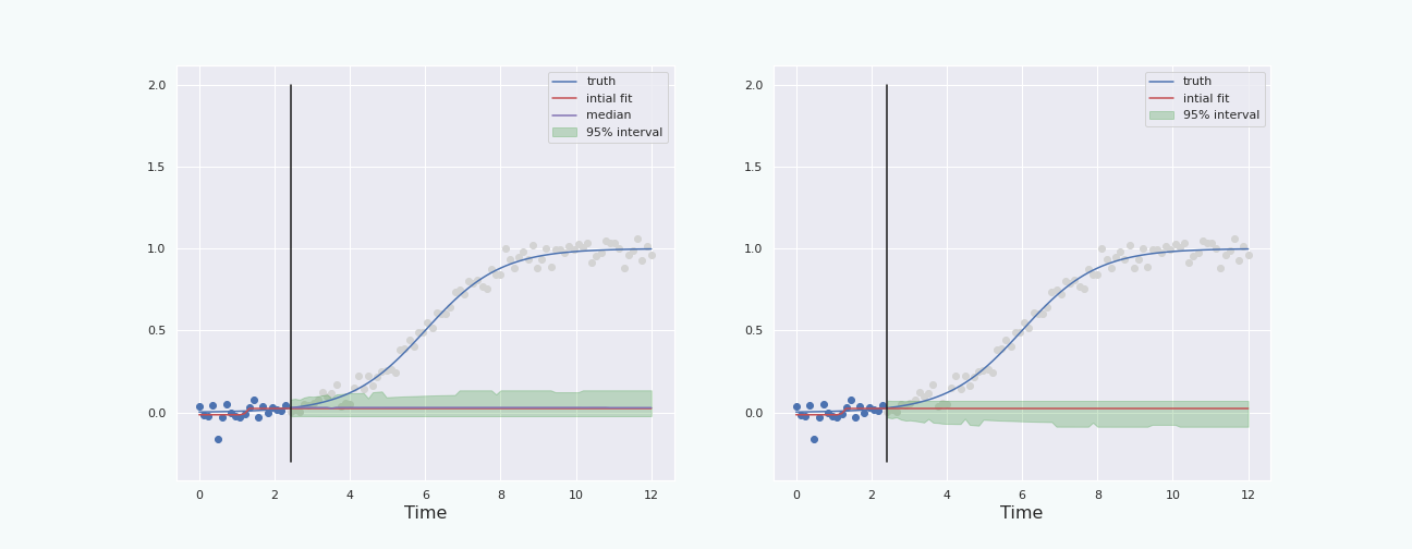
Here we try to predict the expectation values of the future values of the sigmoid+noise given the past values that we observe. There is one prediction for each of the future time step. For each time step, the expected value of the future data at this time step will be considered as a parameter \(\theta\). Let us focus on only one of the time steps, ie only one future data point. To build the confidence interval for this future data point, we proceed as follows:

1. Use the \(k\) past points, and fit the sigmoid to these past points.
2. Use the sigmoid we found in the previous step and store the predicted value at the time step of interest.
3. Generate new data by adding noise to the sigmoid you got in step 1. for all the past time steps. We can do this since we know the probability distribution of the noise we want to add.
4. Fit a new sigmoid to the newly generated data, and record the prediction of this sigmoid on the future time step in a list. Repeat steps 3. and 4. many times.
5. When having a sufficiently long list of predicted values for the time step of interest, find the \(\bar \alpha/2\) percentile and the \(1-\bar \alpha/2\) percentile of the list. These two values will be the lower- and upper-bound of the confidence interval on the predicted value for this time step.

Once you have done this for one future time step, do all the above for the next time steps until you are finished. As you can see in the above procedure, the prediction given at a time step by the fit of the data plays the role of the predicted parameter \(\hat \theta\) we talked about in the previous section, while the value of the true sigmoid at a time step plays the role of the true value of \(\theta\) from the previous section.

Limitations of this method for constructing confidence interval

The most obvious limitation of this method, is that we used the fact that the probability distribution of the noise is known. In practice this is not always the case. In the next section we will see how to remedy this particular issue.

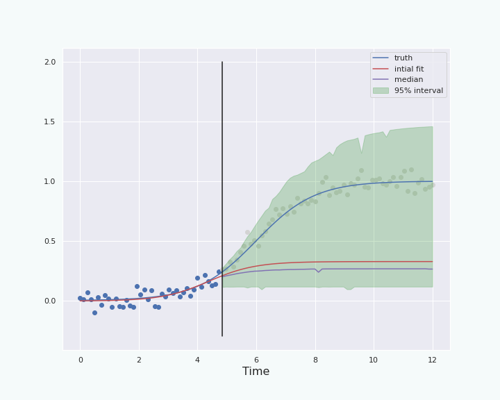
Percentile interval with bootstrap sampling.

In this section we will adapt the above percentile interval construction to the case where we do not know the probability distribution of the noise. To do so, we only have to replace how to generate new data point. In the previous section, we could generate new data in step 3 because we knew how the noise was distributed. So we will modify this step of the procedure, and use bootstrap sampling to generate new data.

Bootstrap sampling.

Bootstrap sampling is a method that allows us to use known data to generate “new” data that approximately follows the same distribution as the known one. Let us consider a list of independent random variables \(X_1, \ldots, X_k\), all following the same unknown probability distribution. The realizations \(x_1, \ldots, x_k\) of these random variables will represent known data. We will now use \(x_1, \ldots, x_k\) to generate what looks like a new list \(\bar x_1,\ldots, \bar x_k\) of realizations of the same random variables \(X_1, \ldots X_k\).

To do so, we will sample uniformly at random (with replacement) elements of the known data to create the new data. In other words, for every \(1\leq i \leq k\) we choose \(\bar x_i := x_{\textrm{rand}(1,k)}\), where the function \({\rm rand}(1,k)\) picks an integer in \([1,k]\) uniformly at random (with replacement). In python this looks like the following (for \(k=50\)):

import numpy as np
k = 50
# Known data: For the example we generate an array of random numbers lying in [0,1[
X = np.random.random(size = k)
# Knew data
X_new = np.random.choice(X, size = k, replace = True)

Back to our problem

We now replace the step 3. of the procedure presented in the previous section. In our new point 3 we will use bootstrap sampling to generate new data. Let us divide the new step 3. into two sub-steps as follows:

1. 1. Compute the list of the differences between the past data points and the value given by the sigmoid obtained in step 1. This is called the residues, and it approximates the noise.
   2. Generate new data by adding to the sigmoid obtained in step 1. the residues picked uniformly at random (with replacement) from the list of residues computed in the previous sub-step. This is the bootstrap sampling of the noise.

All the other steps of the procedure presented in the previous section remain unchanged.

Limitations of this method to construct confidence interval

In this section we have solved the problem of the technique presented in the previous section, namely we can now construct a confidence interval even if we do not know the probability distribution of the noise. However, the method is not perfect and suffers from a few problems either linked to the bootstrap sampling or to the percentile method itself.

1. The bootstrap sampling is only an approximation that does not always work. For example, if one wants to generate more “new points” than one has “old points”, then some of the old point will be picked several times as new point: Some extra correlation appears, therefore the probability distribution of the bootstrap sample is not independently and identically distributed.
2. There is no strong theoretical justification of why percentile confidence interval works: “It just does” [Sec. 5.4, Hest14].
3. In general, this method is not robust when the probability distribution of the noise is skewed or the estimator \(\hat \theta\) is biased [Hest14].

In the following section we will see a method using bootstrap sampling that is in general less sensitive to skewness of the distribution, at least for some estimator (see [Sec. 5.5 & 5.6, Hest14] for more details).

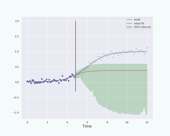
Bootstrap-T (or Boot-T) interval

In this section we will use a method that is often more robust than the previous ones. However, the method is not a magical solution: There are some estimators for which Boot-T performs well, and some others for which it performs poorly. For the purpose of this blog post we will simply use it and compare the result to the previous method.

How to construct the Boot-T interval?

Once again let us call \(\theta\) the parameter we want to estimate, and \(\hat \theta\) an estimator of \(\theta\). The Boot-T interval uses a statistics called the t-statistics:

where \(\hat S\) is an estimator of the standard deviation of \(\hat \theta\).

However, we do not have direct access to the distribution of \(\hat \theta\) and \(\hat S\), therefore we don’t have access to the distribution of the \(t\)-statistics. We will therefore use bootstrap sampling to approximate the distribution of the \(t\)-statistics, similarly as we did approximate the noise distribution with bootstrap sampling in the previous section. In other words, we compute many times the following quantity,

where \(\hat \theta^*\) denotes the estimation of \(\theta\) done through bootstrap sampling, and \(\hat S^*\) is the standard error of \(\hat \theta^*\). We compute this \(t^*\) many times, and store all this values in a list. We can then compute the \(\bar \alpha\) percentile \(q_{\bar \alpha}\) and the \(1-\bar \alpha/2\) percentile \(q_{1-\bar \alpha/2}\) of this list of values of \(t^*\), where \(\bar \alpha = 1-\alpha\), and \(\alpha\) is the confidence level of the interval we are trying to construct as in the previous sections. Then by definition of the percentile we have:

where in the first equation with the \(\approx\) symbol we assume that the bootstrap probability distribution of \(t^*\) is a good approximation of the true distribution of \(t\), and in the second equation with the \(\approx\) symbol we assume that \(\hat S^* \approx \hat S\), ie that the standard error of the estimation \(\hat \theta\) is well approximated by the standard error of the bootstrap estimation \(\hat \theta^*\). The last equation leads to the conclusion that the \(\alpha\)-confidence interval is given by,

This interval is the boot-T confidence interval (for a level of confidence \(\alpha\)). As we can see in this interval the \(1-\bar \alpha/2\) percentile is related to the lower-bound of the interval and the \(\bar \alpha\) percentile is related to the upper bound of the interval. In the percentile intervals of the previous sections the situation was reversed, and we will see in the comparison section that this makes look like the boot-T interval is a sort of mirror image of the percentile interval.

Back to our problem

To use the boot-T confidence interval in our problem we need to follow the following procedure: Let us consider a single time step in the future for which we want to make a prediction. Let us call \(\theta\) the expected value of the future data point at this time step.

1. Use the \(k\) past points, and fit the sigmoid to these past points.
2. Use the sigmoid we found in the previous step and store the predicted value \(\hat \theta\) at the future time step.
3. 1. Compute the list of the differences between the past data points and the value given by the sigmoid obtained in step 1. for these past time steps. These are called the residues, and them approximate the noise.
   2. Generate new data by adding to the sigmoid obtained in step 1. the residues picked uniformly at random (with replacement) from the list of residues computed in the previous sub-step. This is the bootstrap sampling of the noise.
4. Fit a new sigmoid to the newly generated data (on the past time steps), and record the prediction \(\hat \theta^*\) of this sigmoid for the future time step in a list. Repeat steps 3 and 4 many times.
5. When having a sufficiently long list of predicted values for the future time step, compute the standard deviation \(\hat S^*\) of this list. Create a new list whose elements are the t-statistics computed from each element \(\hat \theta^*\) of the previous list and their standard deviation \(\hat S^*\) and the prediction \(\hat \theta\) given in step 2. In this list of t-statistics find the \(\bar \alpha/2\) percentile \(q_{\bar \alpha/2}\) and the \(1-\bar \alpha/2\) percentile \(q_{1-\bar \alpha/2}\). The interval is then given by \(\big [\hat \theta - q_{1-\bar \alpha/2}\hat S^*, \hat \theta -q_{\bar \alpha/2} \hat S^*\big]\).

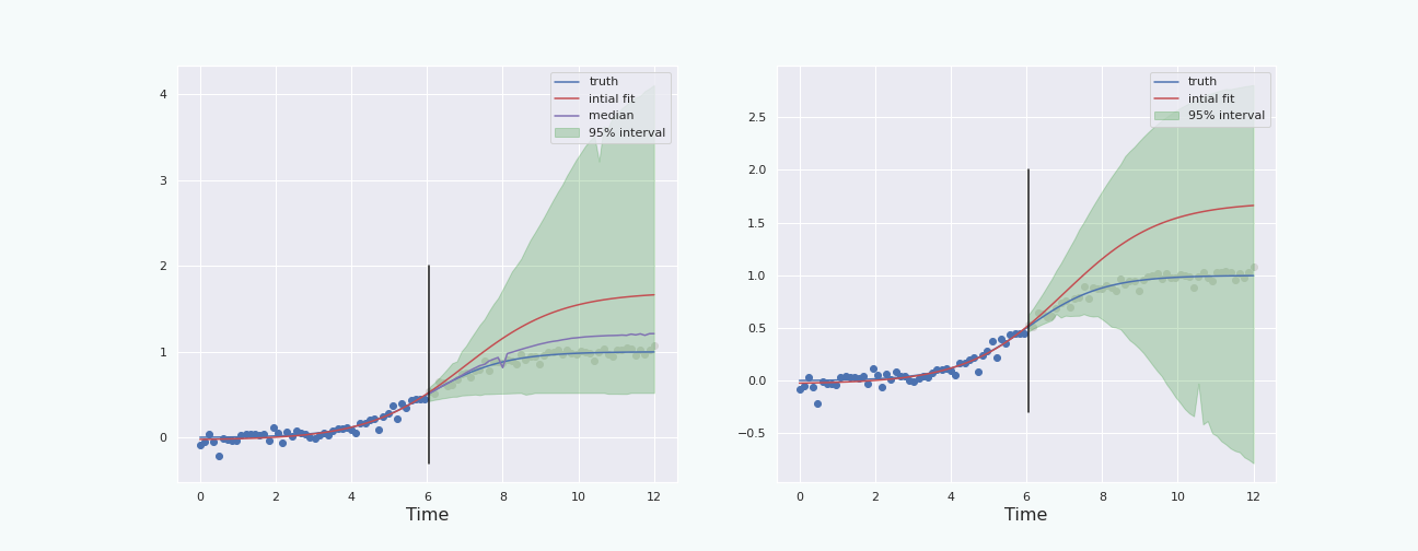
This procedure leads to the following graph.

Interval based on McDiarmid inequality

In this section we will quickly see the possibility to derive confidence interval from some theoretical bound from probability theory. However, we will not spend too much time on this method because it gives larger intervals than the previous methods, and require some not necessarily valid assumptions to be derived.

The McDiarmid inequality is a concentration bound that quantifies by how much certain random variables can deviate from their expectation values. The statement of this inequality goes along the following lines.

Consider independent random variables \(X_1, X_2, \dots X_k\) and a mapping \(f: \mathcal{X}_1 \times \mathcal{X}_2 \times \cdots \times \mathcal{X}_k \rightarrow \mathbb{R}\). Assume there exist constants \(c_1, c_2, \dots, c_k\) such that for all \(i\), \(\underset{x_1, \cdots, x_{i-1}, x_i, x_i', x_{i+1}, \cdots, x_k}{\sup} |f(x_1, \dots, x_{i-1}, x_i, x_{i+1}, \cdots, x_k)-f(x_1, \dots, x_{i-1}, x_i', x_{i+1}, \cdots, x_k)|\leq c_i.\) (In other words, changing the value of the \(i\)th coordinate \(x_i\) changes the value of \(f\) by at most \(c_i\).) Then, for any \(\epsilon > 0\), \(\Pr\big(\big|f(X_1, X_2, \cdots, X_k) - \mathbb{E}[f(X_1, X_2, \cdots, X_k)]\big| \geq \epsilon\big) \leq 2 \exp \left(-\frac{2 \epsilon^2}{\sum_{i=1}^{k} c_i^2}\right).\)

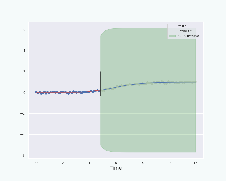
From this we can derive a confidence interval by remembering that the estimator \(\hat \theta\) of the parameter \(\theta\) is a function of the observed data, ie we have \(\hat \theta = f(X_1, \ldots, X_k)\). Skipping all the details, know that under some assumptions we can derive a confidence interval that leads to the following graph.

Comparison & conclusions

Comparison

In this post, we have seen the percentile interval, the boot-T interval and an interval coming from the McDiarmid inequality. Since the last one gives result that are far too loose compare to the others, we will not compare it with the other methods.

In the case of the percentile interval we will only focus on the situation in which the probability distribution of the noise is unknown.

To have a fair comparison, let us plot the percentile interval and the boot-T interval computed on the same data.

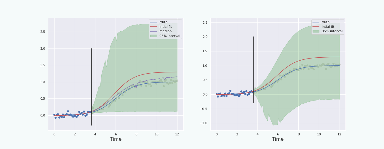
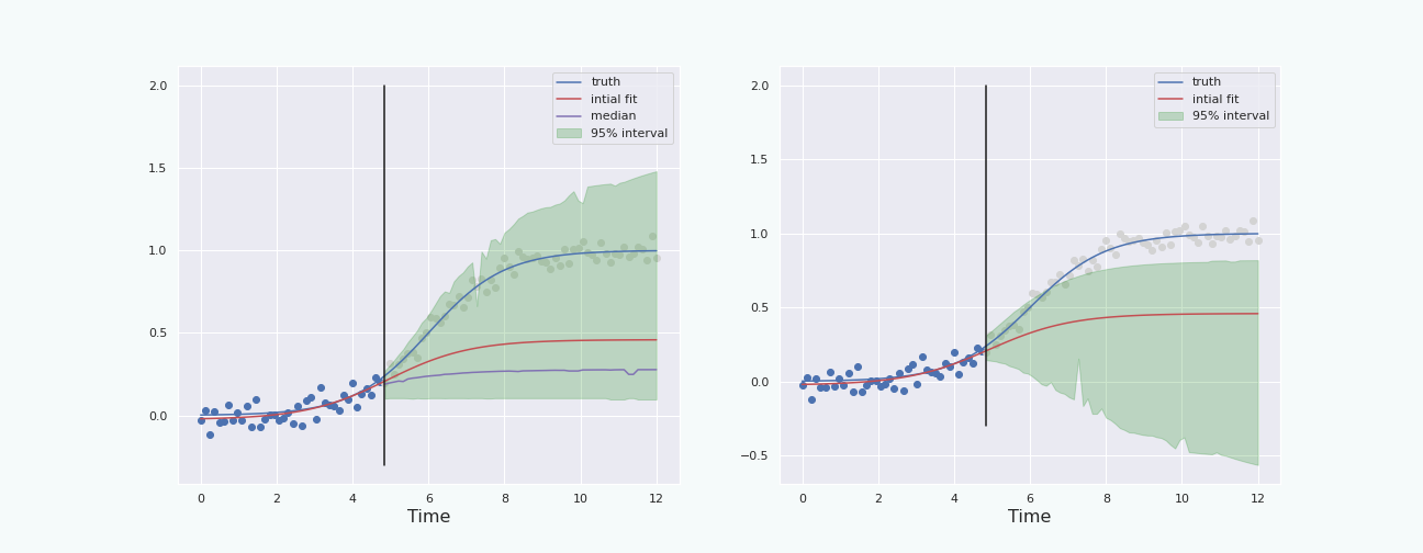
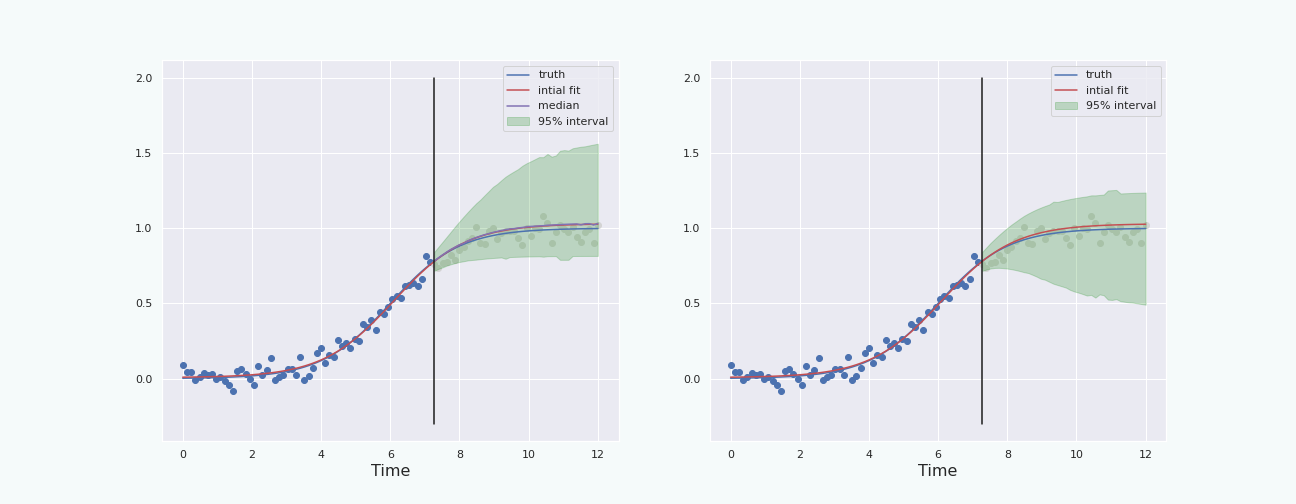
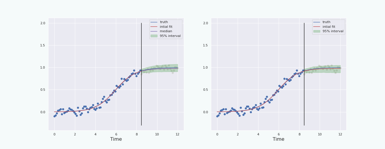
Note that the boot-T interval is basicaly a mirrored image of the percentile interval with respect to the red curve.

Conclusion

The last section shows that, in this particular situation, and with this particular noise, the bootstrap percentile interval behaves better than the boot-T interval. We also see that the interval starts to behave properly (ie it contains the true curve) when the “past data” represents about \(30\%\) and more of the total data, ie when the “future” starts a bit before the inflection point of the sigmoid. This is because at about \(30\%\), the height of the (true) curve starts to become larger than the standard deviation of the noise.

Going further, and possible improvements

If one wants to go further, here are some interesting leads:

1. One can explore the effect of other type of noise on the different techniques to build these intervals. In this post we limited ourselves to Gaussian noise, which is symmetric and with thin tails. It is possible that skewed noise with fat tail distribution can completely change how well the techniques perform in constructing a confidence intervals.
2. An important observation to make about the different plots presented in this post, is that the quality of the fit on the past data completely conditions the quality of the confidence interval. A fit that is too far from the truth on the past data likely leads to an interval that is completely off. Therefore, one may explore the effect of randomization and averaging (using some bootstrap sampling methods) of the fit for the past data to see whether it can improve its quality. This will not only allow to have better confidence intervals, but also get meaningful confidence intervals using less past data.
3. One may want to use another predictor instead of the fit presented here. For example one might want to use the median or the average of an ensemble of fits.
4. A combination of the above is likely to improve the construction of the confidence intervals presented in this post.

A quick word about confidence level

It is easy to be confused by the meaning of a confidence level. One might be tempted to see it as the probability that the true values of the parameter we try to estimate lies in the interval. Rather it is, for a given true value of the parameter and for a given method to construct the interval, the probability that the data leads to the construction of an interval that contains the true value. In other words it measures the capacity that the construction of the interval has to “capture” the true value of the parameter.

References

[Hest14] Hesterberg, Tim C. “What teachers should know about the bootstrap: Resampling in the undergraduate statistics curriculum.” The American Statistician 69.4 (2015): 371-386.