Detecting Disasters on Twitter!
A Natural Language Processing (NLP) project using the pretrained BERT model
Jeremy Ribeiro, 27 December 2020
All the code I have used for this project can be found in this Jupyter Notebook.
In this blog post I will present a Kaggle based NLP project (see the project on Kaggle https://www.kaggle.com/c/nlp-getting-started/overview). The project is the following. We are given a data set containing tweets and some extra information about them. These tweets are labeled according to whether or not they speak about disasters. The goal of the project is simple: Making a model that automatically classifies tweets into the category “it speaks about a disaster” or “it does not speak about a disaster”.
To do that I will use the pretrained BERT model, created by Google, that allows to extract the meaning of words. What it does is that it transforms words into 768-dimensional vectors, such that the vectors of words with similar meaning are somewhat close to each other. On top of this BERT layer, I will add two dense layers that are there to learn the classification task. I’ll explain the training procedure, and the interest of using a pretrained layer.
I will also use more traditional machine learning algorithms and methods to perform this task by first trying to create features form the tweets, and then machine learning from these features. These features are features of the tweets that are not explicit in the tweets, like the mean word length of a tweet for example. For this reason I will call the features meta-data in the following.
I will later explain how to combine the BERT based model and the meta-data based classifiers to try to improve the overall performance of the model. To do so, I will briefly explain a few approaches and develop a little more about the “stacking” strategy I use.
I am using the occasion of this post to also explain some strategies and libraries one can use to try to understand what the model is doing, and why it classifies tweets the way it does.
But first things first. Let me start by presenting the data to you, and how one can clean the data before it is used in the machine learning models.
Table of content
- Data & metrics
- Classification using meta-data only
- Classification using the pretrained BERT model
- Combining the BERT model with meta-data based model
- Inegrate the whole model into a pipeline
- Conclusion
Data & metrics
I use the data provided by Kaggle. After downloading the data, and in order to have an idea of what the data looks like, let’s run the following in python.
data_set = pd.read_csv('./train.csv')
test_set = pd.read_csv('./test.csv')

data_set.head()
From which we get the following output:
| id | keyword | location | text | target | |
|---|---|---|---|---|---|
| 0 | 1 | NaN | NaN | Our Deeds are the Reason of this #earthquake M... | 1 |
| 1 | 4 | NaN | NaN | Forest fire near La Ronge Sask. Canada | 1 |
| 2 | 5 | NaN | NaN | All residents asked to 'shelter in place' are ... | 1 |
| 3 | 6 | NaN | NaN | 13,000 people receive #wildfires evacuation or... | 1 |
| 4 | 7 | NaN | NaN | Just got sent this photo from Ruby #Alaska as ... | 1 |
As you can see the data contains 5 columns, and one of them is the target label: The target label is equal to \(1\) whenever the tweet is about a disaster, and is equal to \(0\) otherwise. We already see that in some columns that there are some NaN values that we will have to take care during the cleaning phase of the data. To make sure that the NaN values are only in the columns ‘keyword’ and ‘location’ we can simply count all the NaNs for each column, and we get the following:
| Feature | number of NaN |
|---|---|
| id | 0 |
| keyword | 61 |
| location | 2533 |
| text | 0 |
| target | 0 |
The shape of the data set is (7613,5). This means that the data set contains 7613 samples (the tweets). For each of them we have 4 features and the target column. Let us check how many of those samples are in each class (“class” here refers to the target value):
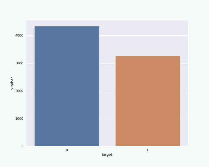
We can see a small imbalance (40:60) between the two classes, but it is not too bad to work with.
Now that we have an idea of the data we have, let’s talk about what metric we will use to measure the predictive power of the model.
Metrics
In order to assess the quality of the model, we need to choose a metric. The Kaggle project page suggests using the so called f1 score. Let us see what is this score and why it is a good metric.
The f1 score is an aggregation of two other metrics called the recall and the precision. To explain what these metrics are let us look at the following figure.

The figure schematically represents all the tweets of the data set: Each dot represents a tweet. When green, the dot represents
a tweet talking about a disaster, otherwise it is red. The goal of the model is to automatically recognize the
tweets talking about a disaster by “reading” them, ie it should be able to find the green dots. The following figure represents the
possible outcome of a model.

We can define what
the recall and precision are using the example of Figure 3. The recall (or recall score) is the fraction of green dots that are in the
circle (ie correctly classified): In Figure 3. it would be \(100\%\) since all the green dots are in the
circle. The precision is the fraction of dots in the circle that are green: In Figure 3. it would be less than \(50\%\) since most of the dots in the
circle are red.

Ideally, we would like a model to have a high recall and a high precision. In order to deal with
a unique number, one can aggregate these two metrics into a single one. The f1 score is such an aggregation of
the recall and the precision. In particular the f1 score is defined as being the harmonic mean of the recall and the precision, ie
if we call the recall \(R\) and the precision \(P\), then the f1 score is defined as,
For example, the illustration of Figure 5. depicts a model with a high f1 score, ie with a high recall and a high precision.

You might now wonder why we pick an expression relatively complicated to aggregate the precision and the recall. Indeed, one could for example, choose to simply compute the arithmetic mean \(\tfrac{R+P}{2}\) of the recall and the precision. This is indeed a possibility, but the arithmetic mean as the inconvenience that its value does not depend on the difference between the recall and the precision: the arithmetic mean will be the same when \((R,P)=(1,0)\) and when \((R,P)=(0.5, 0.5)\). On the other hand, the f1 score can be seen as the arithmetic mean to which we add a penalty term that depends on the difference of \(R\) and \(P\). Indeed, the above expression of the f1 score can be rewritten as,
\[f1 = \frac{R+P}{2}-\frac{(R-P)^2}{2(R+P)}.\]This allows the f1 score to better represent the quality of a model: Having a very good precision but a poor recall will be more penalized than by merely using the arithmetic mean.
Moreover, the f1 score is not very sensitive to imbalanced data (one class of the classification being more represented in the data than the other, like in Figure 1.), as opposed to some other metrics, like the accuracy. This is yet another advantage when dealing with imbalanced data, as we are doing here.
Now that we understand the metric that we will use to assess the model, let’s move on to the cleaning procedure of the data set.
Cleaning process
I will now explain how to perform the cleaning process of the tweets. Indeed, text data, and in particular tweets, are too messy to be used as is in a model. We need to “standardize” as much as possible the text that will be used as input to the model. For example, the following tweet,
only had a car for not even a week and got in a fucking car accident .. Mfs can’t fucking drive .
becomes after cleaning,
only had a car for not even a week and got in a fucking car accident . . mfs cannot fucking drive .
Or the following,
.@NorwayMFA #Bahrain police had previously died in a road accident they were not killed by explosion https://t.co/gFJfgTodad
becomes
. @ norwaymfa # bahrain police had previously died in a road accident they we are not killed by explosion url
In these two examples, we see that all capital letter have been set to lower case fonts, punctuation has been separated from the words, contraction (eg. can’t, shouldn’t…) are expanded (cannot, should not…), the ‘@’ symbol and the ‘#’ symbol are also separated from the words. Moreover, our modification should include some common typo corrections, split some word glued together (eg ‘autoaccidents’ -> ‘auto accidents’), etc.
But how do we know what transformation to make, which typos to correct, and which “glued words” to split?
The strategy here is to use an embedding model (like GloVe or FastText) or a vocabulary list that already exists, and see how many words in the tweets can be found in the embedding or the vocabulary list. Let me now define the “text coverage” and the “vocabulary coverage” as follows:
- vocabulary coverage: It is the fraction of unique words of the text (the tweets) that can be found in the embedding or vocabulary list.
- text coverage: It is the fraction of (not necessarily unique) words of the text (the tweets) that can be found in the embedding or vocabulary list.
For example, let us say that we look at the following text: “The first President of the United States is GeorgeWashington”. The 8 unique words in this text are (we lower case all the words for simplicity): “the”, “first”, “president”, “of”, “united”, “states”, “is”, “georgewashington”. Let us assume that the vocabulary list we use contains the following words: “the”, “first”, “president”, “of”, “united”, “states”, “is”, “george”, “washington”. Among the 8 unique words of the text, 7 can be found in the vocabulary list, since “georgewashingtion” is not in this list. Therefore, the vocabulary coverage in this example is \(7/8 = 0.875\). On the other hand, there are 9 words in the text (since the word “the” appears twice), and 8 of them are in the vocabulary list, so the text coverage is \(8/9 \approx 0.89\).
The goal of the cleaning procedure will be to transform the text so that the text and the vocabulary coverage become as close as possible to \(1\). In the above example, one only needs to split “georgewashington” into “george washington” in order to make both the text coverage and vocabulary coverage equal to \(1\). To do so, we need to find all the words in the text that are not in the vocabulary list, sort them from the most frequent to the least frequent, and make the necessary changes in the cleaning function so that the text coverage and vocabulary coverage increase. You can find some code about this cleaning process in the section 4 of this notebook on Kaggle.
Personally, I merely reuse the cleaning function created by the author of the above mentioned notebook on Kaggle. I modified this function so that it runs faster and so that it generalizes more easily to other text data set. I do so by using the power of regular expressions more extensively. You can find my cleaning function on my own notebook.
Feature extraction: adding meta-data
We will now see that from the raw tweet one can extract some features that are not explicit in the text body (here the tweets). This meta-data can be used for checking that the training set and the test set have the same statistics. Indeed, if this weren’t the case, then there are chances that the learning on the training set poorly generalizes on the test set. On the contrary, if they have similar statistics for several of these features then one can be more confident that the model will give good results on the test set. It is therefore a good sanity check to do before even starting to work on the model.
On the other hand, the statistics of these features might be slightly different for the tweets that speak about disasters compared to the ones that do not. If this is the case, then one could use this meta-data and leverage these differences in the statistics to develop a model classifying the tweets.
I find this idea interesting so let us first try to classify the tweets using the meta data only. I will develop more about the models I used for that in the next section. Let me now tell you what features I have extracted from the tweets. Several of these features are presented in this Kaggle notebook, and others have been added by myself. In total, I have extracted 15 features:
- The number of hashtags of a tweet.
- The number of capitalized words in a tweet
- The number of words of a tweet
- The number of unique words of a tweet
- The number URLs of a tweet
- The mean word length of a tweet
- The number of characters of a tweet
- the number of punctuation characters of a tweet
- The number of mentions of a tweet
- The number of mentions of a tweet that can be found in tweets of the training set labeled as ‘tweet talking about a disaster’. The idea is that, some mentions might be particularly frequent in the tweets talking about disasters. One can think about mention of newspapers’ accounts etc.
- The number of mentions of a tweet that can be found in tweets of the training set labeled as ‘tweet not talking about a disaster’. The idea is the same as above, but with the tweets that do not talk about a disaster.
- The difference between the last two features.
- The number of 2-grams of a tweet that are among the top 100 2-grams in tweets of the training set labeled as ‘tweet talking about a disaster’
- The number of 2-grams of a tweet that are among the top 100 2-grams in tweets of the training set labeled as ‘tweet not talking about a disaster’. The idea of this feature and the previous one is that some 2-grams can be more frequent in “disaster tweets” and other 2-gram more present in “none disaster tweets”.
- The difference between the last two features
One needs to be very careful when writing the code that will extract these features: Some of them (the features 10, 11, 13, and 14) use the labels (‘target’ feature of the data set) of the training set in order to extract the relevant information. You should allow your code to use the labels on the training set only, not on the validation set. Not paying attention to that can result in a label leakage (aka target leakage) which Wikipedia defines as follows:
In statistics and machine learning, leakage (also data leakage, or target leakage) is the use of information in the model training process which would not be expected to be available at prediction time, causing the predictive scores (metrics) to overestimate the model’s utility when run in a production environment.[1] Leakage is often subtle and indirect, making it hard to detect and eliminate. Leakage can cause modeler to select a suboptimal model, which otherwise could be outperformed by a leakage-free model.[1]
In order to avoid this issue, one needs to split the data set into a training set and a validation set before adding any feature:
X_train, X_val, y_train, y_val = train_test_split(data_set[['keyword','text', 'text_cleaned']],
                                                  data_set['target_corrected'])
Then for the steps that use the labels of the training set one needs to make use of transformers like the ones provided by the library scikit-learn. Let’s see a code example of that:
# Create the transformer object of the class CountMentionInClass().
# This class is a customized version of a scikit-learn transformer that I have programmed for
# creating the above mentioned features 10 and 11.
mentionCounter = CountMentionsInClass()

# Create and add the features 10 and 11 to the training set X_train.
# Note that the fit_transform() method uses the labels stored in y_train
X_train = mentionCounter.fit_transform(X_train, y_train, column='text')

# Create and add the features 10 and 11 to the validation set X_val.
# Note that the transform() method does not use any label.
X_val = mentionCounter.transform(X_val, column='text')
The code for the definition of the CountMentionInClass class can be found in the MyClasses.py file here. Splitting the data set before adding the features, and by using transformers as shown above, allows to reduce the risk of a label leakage. It has the additional advantage that the code written like this can easily be included into a pipeline as we will see later in this post.
Classification using meta-data only
Once the meta-data features are created one can try to use these in order to classify the tweets. I will quickly present two models for that: One using Random Forest and one using Logistic Regression. For these two models I will present ways of trying to interpret the model. In particular, I will present a method to see what features are important for the model. Then I will present a method that allows to interpret a classification done by the model, ie we will try to answer the following question: Given a tweet, why did the model “decided” to classify it the way it did?
In both cases we will use X_train (shape=(5709, 18)), y_train as training data, and we will use X_val (shape=(1904, 18)), y_val for assessing the model. We will consider that all the meta-data features have already been added to this training data. By running the following
X_val.head(3)
we get,
| keyword | text | text_cleaned | hastags_count | capital_words_count | word_count | unique_word_count | url_count | mean_word_length | char_count | punctuation_count | mention_count | count_mentions_in_disaster | count_mentions_in_ndisaster | difference_mentions_count | count_2-grams_in_disaster | count_2-grams_in_ndisaster | difference_2-grams_count | |
|---|---|---|---|---|---|---|---|---|---|---|---|---|---|---|---|---|---|---|
| 6447 | suicide%20bombing | @Haji_Hunter762 @MiddleEastEye maybe some muzz... | haji hunter middle east eye maybe some muzzies... | 0 | 1 | 17 | 17 | 0 | 6.941176 | 134 | 13 | 2 | 0 | 0 | 0 | 1 | 0 | 1 |
| 7433 | wounded | @wocowae Officer Wounded Suspect Killed in Exc... | @ wocowae officer wounded suspect killed in e... | 0 | 0 | 11 | 11 | 1 | 7.363636 | 91 | 6 | 1 | 0 | 0 | 0 | 2 | 0 | 2 |
| 4836 | mass%20murder | @yelllowheather controlled murder is fine. mas... | @ yelllowheather controlled murder is fine . ... | 0 | 0 | 16 | 15 | 0 | 5.750000 | 107 | 5 | 1 | 0 | 0 | 0 | 0 | 0 | 0 |
As you can see there are 18 columns. The first two were already present in the data set1, then follows the cleaned tweets, and finally the 15 added features. For the classification we will use the first column and the 15 added features, ie the only column I don’t use are the tweets and their cleaned version.
Random Forest
The model I will present in here is based on a random forest classifier. In particular, I will use the random forest classifier from scikit-learn, to which I add some data preparation steps for the features. Note that we have a lot of numerical features, and one categorical feature, and we need to treat them separately in the data preparation steps. Let us then define the following:
# Categorical meta-data
cat_metaData_features = ['keyword']

# numerical meta-data
numerical_metaData_features = ['hastags_count', 'capital_words_count', 'word_count', 'unique_word_count',
                               'url_count', 'mean_word_length', 'char_count', 'punctuation_count',
                               'mention_count', 'count_mentions_in_disaster', 'count_mentions_in_ndisaster',
                               'difference_mentions_count', 'count_2-grams_in_disaster', 'count_2-grams_in_ndisaster',
                               'difference_2-grams_count']
# text feature
txt_feature = ['text_cleaned']
This allows us to quickly refer to the categorical data or to the numerical data. Here, the data preparation will be extremely simple. We will rescale all the numerical feature, so that their standard deviation equals 12. For the categorical feature we need to encode them. For that, I will use the OneHotEncoder from scikit-learn:
# Define the scaling and the encoding
enc_scale = ColumnTransformer([('scaler',StandardScaler(), numerical_metaData_features),
                               ('enc', OneHotEncoder(handle_unknown='ignore'), cat_metaData_features)]).fit(X_train,y_train)

# Define the Random Forest model
Model_Forest = RandomForestClassifier(n_estimators=900, max_depth=23, n_jobs=8, class_weight='balanced')

# Train the model on the data after scaling and encoding.
# In a next section we will see how to use pipelines in order to integrate the model and the data preparation in a single object.
Model_Forest.fit(enc_scale.transform(X_train), y_train)


# Evaluate the model on the training set and on the validation set.
y_train_pred = Model_Forest.predict(enc_scale.transform(X_train))
y_val_pred = Model_Forest.predict(enc_scale.transform(X_val))

# training score
print("Training scores:\n",
      "precision={:.2f}".format(skl.metrics.precision_score(y_true=y_train, y_pred=y_train_pred)),
      "recall={:.2f}".format(skl.metrics.recall_score(y_true=y_train, y_pred=y_train_pred)),
      "f1={:.2f}".format(skl.metrics.f1_score(y_true=y_train, y_pred=y_train_pred))
      )

# validation score
print("\nValidation scores:\n",
      "precision={:.2f}".format(skl.metrics.precision_score(y_true=y_val, y_pred=y_val_pred)),
      "recall={:.2f}".format(skl.metrics.recall_score(y_true=y_val, y_pred=y_val_pred)),
      "f1={:.2f}".format(skl.metrics.f1_score(y_true=y_val, y_pred=y_val_pred))
      )
By running the above code we obtain the following output.
Training scores:
precision=0.81 recall=0.91 f1=0.86
Validation scores:
precision=0.60 recall=0.74 f1=0.67
To have an idea of how well the model performs, one should look at the f1 score for the validation set, since it should tell us what would be the score on truly new data. Printing the f1 score of the training set can be useful: If it is too high compared to the score on the validation set, then the model might overfit the data. Overfitting can hurt the performance of the data, so it is important to detect it. Here, the training score is 0.86 while the validation score is 0.67. There is probably some overfitting here. I suspect that this is due to the added features 10, 11, 13, and 14, which by construction “memorize” some text specific of the training set. It would be worth exploring this further to see whether the performance of the model can be improved. However, for the purpose of this post, I won’t do that. Instead, I’ll move on to the model explanation, which can actually be part of the required work for improving the model and reducing the overfitting. Indeed, Model explanation is a tool meant to diagnose issues with the model.
Besides, it can also be used to justify the “decision” made by the model for any given example provided as input. You might want to do that to convince yourself, or maybe to convince others, that the model is doing something that makes sense, and that it can therefore be trusted.
Model explanation
In order to explain the model I will use the eli5 library, that is a library specialized into model explanation. Let’s start with Feature Importance. Feature Importance is simply a measure of the importance of each feature for the model. Here, I will use what is called Permutation Importance. Permutation Importance compute the importance of a feature as follows.
- Apply the model on the validation set, and evaluate the performance of the model.
-
- Pick a column of the validation set (X_val), randomly permute the values of the column.
- Apply the model on the validation set (on which the column has been permuted), and evaluate the new performance of the model.
- Permute the column back to recover the original validation set.
- Perform step 2 for all the columns of the validation set.
Once this is done, you can see by how much the performance has change after the permutation of a column compare to the initial performance on the original set. This difference is the permutation importance of the column.
Intuitively, randomly permuting a column basically erases all the correlations between the values of this column and the values of the target (stored in y_val). In terms of information, it is as if you erased the information contained in the column. We then expect that, the more a feature (column) is important for the model, the more the model performance drops after the permutation of this feature.
The operation I have described above is automatically performed by the PermutationImportance class of the library eli5:
##### First redefine and train the Random Forest model in a way that will be accepted by the PermutationImportance class.

# copy X_train into X
X = X_train[cat_metaData_features+numerical_metaData_features].copy()
X[cat_metaData_features] = OrdinalEncoder().fit_transform(X[cat_metaData_features])

# The model is the same as before, but integrated into a pipeline. It is fitted on the same training set X_train (X is used as a proxy for X_train).
model_metadata = make_pipeline(enc_scale, Model_Forest).fit(X[cat_metaData_features+numerical_metaData_features], y_train)


##### Feature importance: permutation importance

# copy X_val into X
X = X_val[cat_metaData_features+numerical_metaData_features].copy()

# Have to use OrdinalEncoder() because PermutationImportance() will internally try to convert
# the categories into floats (idk why...), and it will fail if I keep the categories as strings
X[cat_metaData_features] = OrdinalEncoder().fit_transform(X[cat_metaData_features])

perm_importance = PermutationImportance(model_metadata).fit(X, y_val)  # performs the operations I have described above.
eli5.show_weights(perm_importance, feature_names=cat_metaData_features+numerical_metaData_features)  # display the importance of each feature in a table
After running the above code we get the following table.
| Weight | Feature |
|---|---|
| 0.0243 ± 0.0114 | mean_word_length |
| 0.0203 ± 0.0084 | keyword |
| 0.0196 ± 0.0073 | difference_2-grams_count |
| 0.0098 ± 0.0102 | char_count |
| 0.0084 ± 0.0051 | count_2-grams_in_ndisaster |
| 0.0082 ± 0.0030 | count_2-grams_in_disaster |
| 0.0045 ± 0.0021 | count_mentions_in_disaster |
| 0.0043 ± 0.0045 | capital_words_count |
| 0.0035 ± 0.0039 | difference_mentions_count |
| 0.0024 ± 0.0044 | count_mentions_in_ndisaster |
| 0.0017 ± 0.0038 | punctuation_count |
| 0.0007 ± 0.0014 | hastags_count |
| -0.0001 ± 0.0031 | mention_count |
| -0.0019 ± 0.0053 | url_count |
| -0.0044 ± 0.0042 | word_count |
| -0.0054 ± 0.0050 | unique_word_count |
We see that for this model, the three most important features are “mean_word_length”, “keyword”, “difference_2-grams_count”. The weights associated to each feature is the amount by which the performance of the model drops.
The above tells us how important each feature is for the model, by looking at the whole validation set. There are at least two pieces of information about which it says nothing: It does not allow to explain the predictions of the model for an individual sample of the data set, and does not tell in which direction a given feature influences the prediction, it only says whether it will have a big influence. Eli5 gives some methods to explain the model with these two extra pieces of information. However, because of the one hot encoding, our model is not supported by these explainers.
I will therefore use the shap library which gives for every sample of the data set a “contribution score” for each feature. It does so by computing what is called the Shapley value for each feature of a given sample. The Shapley value is a concept that has been developed in the context of game theory. So a priori it has very little to do with model explanation. The Shapley value would deserve a blog post on its own, but in short, the Shapley value is the solution to how to share profit among collaborator based on a notion of “merit”. The notion of merit can be given a precise definition in this game theoretic framework: It roughly says that if an individual contributes more he should get a larger share of the profit. We can already see some analogy with what we intuitively think a “contribution score” of a feature should do. But you might wonder what is the “profit” in our context? It’s actually the difference between the predicted probability given by our model on a given example and a base value which can be thought of the probability the model would predict if it were not given any features. Let us see an example for the following sample,
X_val.iloc[5].loc['text']
'4 kidnapped ladies rescued by police in Enugu | Nigerian Tribune http://t.co/xYyEV89WIz'.
Without diving into how to use the shap library, here is the output we get,

You see that each feature is assigned to a score (positive or negative) depending on the value taken by this feature. The sum of all the Shapley values should be equal to the difference between the base value and the predicted probability. When a score is negative (in blue) it tends to decrease the predicted probability, and vice versa. As expected, we can see that the features with the largest (positive or negative) Shapley value often correspond to the most important features according to the permutation importance: For example, “mean_word_length” has the second largest Shapley value, and it also has the second highest permutation importance. Of course the Shapley values will change for each sample, since each of them has different feature values. To make sure that there really is a correspondence between permutation importance and the Shapley values, one would need to compute the Shapley values of many samples, and then check that the correspondence holds on average over these samples.
Logistic Regression
In this section, we will see the exact same thing as before but by replacing RandomForestClassifier by LogisticRegression. Since the code is exactly the same as before (except for the use of the LogisticRegression) I will simply show the f1 score of this new model.
Training scores:
precision=0.79 recall=0.83 f1=0.81
Validation scores:
precision=0.69 recall=0.75 f1=0.72
All the remark made in the previous section apply here too. The main difference is that this model seems a bit better, and seems to overfit a little less. One thing that is important though, is that for this model the scaling of the numerical values in the data preparation step is more important, so it is crucial not to forget to rescale the numerical features when using logistic regression.
Model explanation
Again, everything we have seen about the model explanation for the random forest model also applies here. Let’s see what we get when computing the permutation importance for the new model:
| Weight | Feature |
|---|---|
| 0.1595 ± 0.0081 | keyword |
| 0.1256 ± 0.0128 | char_count |
| 0.0888 ± 0.0090 | word_count |
| 0.0391 ± 0.0108 | difference_2-grams_count |
| 0.0196 ± 0.0080 | count_2-grams_in_disaster |
| 0.0121 ± 0.0058 | punctuation_count |
| 0.0082 ± 0.0025 | count_mentions_in_disaster |
| 0.0069 ± 0.0035 | difference_mentions_count |
| 0.0065 ± 0.0070 | count_mentions_in_ndisaster |
| 0.0034 ± 0.0019 | count_2-grams_in_ndisaster |
| 0.0027 ± 0.0050 | mean_word_length |
| 0.0027 ± 0.0042 | unique_word_count |
| 0.0020 ± 0.0041 | mention_count |
| 0.0001 ± 0.0008 | url_count |
| -0.0004 ± 0.0046 | capital_words_count |
| -0.0020 ± 0.0015 | hastags_count |
Let us see what the shap library tells us about the following sample,
X_val.iloc[5].loc['text']
'4 kidnapped ladies rescued by police in Enugu | Nigerian Tribune http://t.co/xYyEV89WIz'.
Once the Shapley values are calculated, we get the following,

Here again we can see that the features with high contribution (positive or negative) often are the one with a high permutation importance: For example, here it is true for “word_count” and “char_count”.
Classification using the pretrained BERT model
In this section I will present how to use the BERT model to classify the tweets. As I mentioned earlier, the BERT model is a machine learning model that will map every tweet to a 768-dimensional vector. This vector can be seen as an abstract representation of the meaning of the tweet. In particular, two semantically similar tweets should be represented by two vectors that are close to each other. In other words, the BERT model automatically extracts the meaning of the tweets. Extracting the meaning of the tweets is great, but we still need to perform the classification of these tweets. To do so, I add, on top of the BERT model, two dense layers.
The BERT model has been pretrained by researchers with a ton of data. This means that I only need to train the two dense layers I add on top. This can be done with much fewer data. You can find the pretrained BERT model here.
Let’s now see how to use the BERT model in Python:
# Load the pretrained layer in bert_layer
try:
    bert_layer = hub.KerasLayer("./bert_en_uncased_L-12_H-768_A-12_2/",
                            trainable=False)
except:
    bert_layer = hub.KerasLayer("https://tfhub.dev/tensorflow/bert_en_uncased_L-12_H-768_A-12/2",
                            trainable=False)


# write the function that creates the model based of the BERT layer
def build_bert_model(max_seq_length=80):

    # the BERT model takes as input 3 layers of lengths 80 each.
    input_word_ids = K.layers.Input(shape=(max_seq_length,), dtype=tf.int32,
                                           name="input_word_ids")
    input_mask = K.layers.Input(shape=(max_seq_length,), dtype=tf.int32,
                                       name="input_mask")
    segment_ids = K.layers.Input(shape=(max_seq_length,), dtype=tf.int32,
                                        name="segment_ids")

    pooled_output, sequence_output = bert_layer([input_word_ids, input_mask, segment_ids])
    clf_output = sequence_output[:, 0, :]

    inputs = [input_word_ids, input_mask, segment_ids]
    mid = K.layers.Dense(768, activation='relu')(clf_output)
    out = K.layers.Dense(1, activation='sigmoid')(mid)

    # the class MyModel() is a custom class that inherits from tensorflow.Keras.Model()
    # it allows me to customize the training process.
    model = MyModel(inputs=inputs, outputs=out)
    model.compile(loss='binary_crossentropy', optimizer = 'adam', metrics=['accuracy'])

    return model


# Creates a Model compatible with the scikit-learn API
Bert_model = KerasClassifier(build_bert_model)
You’ll notice that I use the class MyModel in the code. This is a custom version of tf.Keras.Model that allows me to train the model the way I want. In particular, it allows me to check whether there exists a saved model, in which case it simply loads it. Otherwise, it goes to the training of the two dense layers (and only them) I have added on top of the BERT layer by freezing the BERT layer. Then it goes to fine-tuning where I unfreeze the BERT layer and train the whole model for a few epochs. In the following code block is the class that implements the class MyModel that I have coded:
 class MyModel(K.Model):
    """ This class is mostly the same as tensorflow.keras.Model()
    Main changes:
    - fit() method: modified so that, if there is
        a saved model, then load it. Otherwise, train the model in two steps:

        1. Freeze the BERT layer and train only the top layer over 'epochs1' epochs
        2. Unfreeze the BERT layer, and fine-tune the whole model over 'epochs2' epochs

        In the case where the model is trained, the fit method returns the two histories

    - adding _encode() method:
        The _encode() method convert a pandas.Series of strings into an adapted encoding for
        the neural network.

    - adding the predict_classes() method for compatibility with the tensorflow.keras.wrappers.scikit_learn.KerasClassifier()
        wrapper.
     """

    def __init__(self,inputs=None, outputs=None, max_seq_length=80):
        super(MyModel, self).__init__(inputs=inputs, outputs=outputs)
        self.max_seq_length = max_seq_length


    def _encode(self, X):
        X = pd.Series(X)
        X = X.copy()

        max_seq_length = self.max_seq_length
        texts = X.copy()

        vocab_file = bert_layer.resolved_object.vocab_file.asset_path.numpy()
        do_lower_case = bert_layer.resolved_object.do_lower_case.numpy()
        tokenizer = tokenization.FullTokenizer(vocab_file, do_lower_case)

        all_tokens = []
        all_masks = []
        all_segments = []

        for text in texts:
            text = tokenizer.tokenize(text)
            text = text[:max_seq_length - 2]
            input_sequence = ['[CLS]'] + text + ['[SEP]']
            pad_len = max_seq_length - len(input_sequence)

            tokens = tokenizer.convert_tokens_to_ids(input_sequence)
            tokens += [0] * pad_len
            pad_masks = [1] * len(input_sequence) + [0] * pad_len
            segment_ids = [0] * max_seq_length

            all_tokens.append(tokens)
            all_masks.append(pad_masks)
            all_segments.append(segment_ids)

        return np.array(all_tokens), np.array(all_masks), np.array(all_segments)

    def fit(self, x=None, y=None, batch_size=None, epochs1=1, epochs2=1, verbose=1,
        callbacks=None, validation_split=0.0, validation_data=None, shuffle=True,
        class_weight=None, sample_weight=None, initial_epoch=0,
        steps_per_epoch=None, validation_steps=None, validation_batch_size=None,
        validation_freq=1, max_queue_size=10, workers=1,
        use_multiprocessing=False, bert_layer_idx=3):

        x = self._encode(x)

        try:
            # if there is already a saved model use it
            self.load_weights("./weights.best.hdf5")
            self.compile(loss='binary_crossentropy', optimizer = 'adam', metrics=['accuracy'])
            return None
        except:
            # If no saved model, then train the model
            # Start training the top layers of the model with epochs1
            self.layers[bert_layer_idx].trainable=False
            self.compile(loss='binary_crossentropy', optimizer = 'adam', metrics=['accuracy'])
            history1 = super().fit(x=x, y=y, batch_size=batch_size, epochs=epochs1, verbose=1,
                        callbacks=callbacks, validation_split=validation_split, validation_data=validation_data,
                        shuffle=shuffle, class_weight=class_weight, sample_weight=sample_weight, initial_epoch=initial_epoch,
                        steps_per_epoch=steps_per_epoch, validation_steps=validation_steps, validation_batch_size=validation_batch_size,
                        validation_freq=validation_freq, max_queue_size=max_queue_size, workers=workers,
                        use_multiprocessing=use_multiprocessing)

            # Start fine-tuning the model with epochs2
            try:
                self.load_weights("./weights.best.hdf5")  # use the best epoch of the above training if available
            except:
                pass
            self.layers[bert_layer_idx].trainable=True
            self.compile(loss='binary_crossentropy', optimizer = 'adam', metrics=['accuracy'])
            history2 = super().fit(x=x, y=y, batch_size=batch_size, epochs=epochs2, verbose=1,
                        callbacks=callbacks, validation_split=validation_split, validation_data=validation_data,
                        shuffle=shuffle, class_weight=class_weight, sample_weight=sample_weight, initial_epoch=initial_epoch,
                        steps_per_epoch=steps_per_epoch, validation_steps=validation_steps, validation_batch_size=validation_batch_size,
                        validation_freq=validation_freq, max_queue_size=max_queue_size, workers=workers,
                        use_multiprocessing=use_multiprocessing)


            return (history1, history2)

    def evaluate(self, x=None,y=None, batch_size=None, verbose=1, sample_weight=None,
                 steps=None, callbacks=None, max_queue_size=10, workers=1,
                 use_multiprocessing=False, return_dict=False):

        x = self._encode(x)

        return super().evaluate(x=x,y=y, batch_size=batch_size, verbose=verbose, sample_weight=sample_weight,
                 steps=steps, callbacks=callbacks, max_queue_size=max_queue_size, workers=workers,
                 use_multiprocessing=use_multiprocessing, return_dict=return_dict)

    def predict_proba(self, x, batch_size=None, verbose=0, steps=None, callbacks=None,
                max_queue_size=10, workers=1, use_multiprocessing=False):


        x = self._encode(x)

        return super().predict(x, batch_size=batch_size, verbose=verbose, steps=steps, callbacks=callbacks,
                max_queue_size=max_queue_size, workers=workers, use_multiprocessing=use_multiprocessing)

    def predict_classes(self, x, batch_size=None, verbose=0, steps=None, callbacks=None,
                max_queue_size=10, workers=1, use_multiprocessing=False):

        y_pred = self.predict_proba(x, batch_size=batch_size, verbose=verbose, steps=steps, callbacks=callbacks,
                max_queue_size=max_queue_size, workers=workers, use_multiprocessing=use_multiprocessing)

        y_pred = np.array(list(map(lambda b: int(b>0.5), y_pred)))

        return y_pred

    def train_on_batch(self, x, y=None, sample_weight=None, class_weight=None,
                       reset_metrics=True, return_dict=False):

        x = self._encode(x)

        return super().train_om_batch(x, y=y, sample_weight=sample_weight, class_weight=class_weight,
                                      reset_metrics=reset_metrics, return_dict=return_dict)

    def test_on_batch(self, x, y=None,  sample_weight=None, reset_metrics=True, return_dict=False):

        x = self._encode(x)

        return super().test_on_batch(x, y=y, sample_weight=sample_weight, reset_metrics=reset_metrics,
                                     return_dict=return_dict)
    def predict_on_batch(x):

        x = self._encode(x)

        return super().predict_on_batch(x)
Note that when you train your model you can define a callback to, for example, save your model so that next time you can simply load the model instead of retraining everything:
# This is the callback used to save the best model during training.
# If there is no already saved model, then pass this call back
# as an option in the fit method.
best_model = K.callbacks.ModelCheckpoint("./weights.best.hdf5",
                            monitor="val_loss",
                            verbose=1,
                            save_best_only=True,
                            mode='min'
                            )
Finally, in order to have a fully functioning model, I add the cleaning function I have talked about in the beginning of this post as a transformer before my BERT based model,
# BERT classifier pipeline

def clean_text(X):
    X = pd.Series(X)
    X = X.copy()

    return X.apply(lambda s: clean(s))

Cleaner_text = skl.preprocessing.FunctionTransformer(clean_text)

# this is the full model!
Bert_clf = Pipeline([('cleaner_text', Cleaner_text),
                     ('bert_model', Bert_model)

            ])
You can then train the model. Training a model that is as big as the BERT model (in total I have 110,073,602 parameters in my model) is computationally expensive, and it is therefore a good idea to train the model using GPU acceleration. Personally I did it using Google Colaboratory.
The training can be perfromed by executing the following code:
# if you have a saved model, this is enough
Bert_clf.fit(X_train['text'],y_train)

# if you don't have a saved model, then you can use the following
BATCH_SIZE = 32
EPOCHS1 = 20
EPOCHS2 = 5

Bert_clf.fit(X_train['text'],
             y_train,
             validation_data=(X_val['text']), y_val),
             epochs1=EPOCHS1,
             epochs2=EPOCHS2,
             batch_size = BATCH_SIZE,
             shuffle=True,
             callbacks = [best_model]
           )
As for the previous models, once the model is trained, we can print its f1-score to assess its performance:
y_train_pred = Bert_clf.predict(X_train['text'])
y_val_pred = Bert_clf.predict(X_val['text'])

# training score
print("Training scores:\n",
      "precision={:.2f}".format(skl.metrics.precision_score(y_true=y_train, y_pred=y_train_pred)),
      "recall={:.2f}".format(skl.metrics.recall_score(y_true=y_train, y_pred=y_train_pred)),
      "f1={:.2f}".format(skl.metrics.f1_score(y_true=y_train, y_pred=y_train_pred))
      )

# validation score
print("\nValidation scores:\n",
      "precision={:.2f}".format(skl.metrics.precision_score(y_true=y_val, y_pred=y_val_pred)),
      "recall={:.2f}".format(skl.metrics.recall_score(y_true=y_val, y_pred=y_val_pred)),
      "f1={:.2f}".format(skl.metrics.f1_score(y_true=y_val, y_pred=y_val_pred))
      )
Training scores:
precision=0.87 recall=0.80 f1=0.84
Validation scores:
precision=0.88 recall=0.81 f1=0.84
This model clearly beats the previous two models. But is it as interpretable as the meta-data based models? We will see that in the next section.
Model explanation
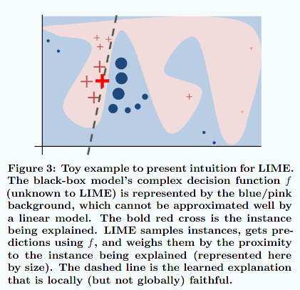
Let us try to interpret the model. The issue here compared to the previous models, is that we don’t have a fixed number of identifiable features for which we can measure an “importance” or a “contribution score”. Fortunately some smart people have already come up with solutions to explain a model like this one. In particular, I will present a tool from eli5 (again) that allows to explain models working on text data. The tool is simply called TextExplainer.
Let me explain quickly what this tool does. For that let me state the obvious: There are very simple models that can be very easily explained, eg linear models are easily explained by their sets of coefficients. However, these simple models are limited. On the other hand, more complex model are more powerful but very hard to interpret. The idea is then to locally approximate complex models by simple ones, and then interpret the simple ones (see Figure 7 from [RSG]). This explanation algorithm is called LIME (Local Interpretable Model-agnostic Explanations). The class TextExplanainer of the library eli5 is an implementation of this algorithm.
Here is an example of how to use the text explainer.
# Explain what the model looks at in a text

# create and fit the text explainer
te = TextExplainer(n_samples=300, position_dependent=True)
text = "10000 people died yesterday. "
te.fit(doc, Bert_clf.predict_proba)

# show the prediction and some metrics that indicates how trustworthy the explanation is
print(te.metrics_)
te.show_prediction()
When running this code, we get the following table and highlighted text as output. It shows the contribution of the words versus bias, and the highlighted text shows the details of the contribution of each word.
| Contribution? | Feature |
|---|---|
| +3.898 | Highlighted in text (sum) |
| -2.703 | <BIAS> |
{'mean_KL_divergence': 0.02224054150605272, 'score': 1.0}
10000 people died yesterday.
Here, two things are present: Some metrics and a highlighted text. The metrics are a measure of how well the linear model approximate the complex model: the closer the “KL divergence” is to \(0\) the better, and the closer the “score” is to \(1\) the better. Here the score are very close to their best values, which indicates that the linear approximation is locally pretty good, and that there are good chances that the model explanation can be trusted.
In the highlighted text we see that the words that contribute the most in the classification are “died” and “people” (you can get the numerical value of the contribution of each word by hovering the words with your mouse).
We can show the importance (the weight) of each word in the text as follows:
te.show_weights()
We then get the following table:
| Weight? | Feature |
|---|---|
| +1.600 | [2] died |
| +1.397 | [1] people |
| +0.614 | [0] 10000 |
| +0.281 | [3] yesterday |
| -2.791 | <BIAS> |
When using text data the difference between the “contribution” and the “weight” of a word should not be very important. Indeed, a word can either be present or not (at a given position of the sentence), but it cannot be “twice as present” than another word. It is therefore not so surprising that the weights (in the above table) and the contribution scores (see the highlighted text above) are similar.
Combining the BERT model with meta-data based model
In this section I will show a way of combining two models that work on two different types of data, in such a way that the combination of these models leads to a better model than each of the model separately. In this particular case, we should not expect a big improvement over the BERT based model. Indeed, all the meta-features are extracted from the text, and since the BERT based model directly uses the text, it has therefore implicit access to the meta-data features. Note that there are still some features that the BERT based model cannot see, like “capital_word_count” since the BERT layer only sees lower-case word and is therefore case-insensitive. However, “capital_word_count” is not a very important feature for the meta-data classifiers and so it should not influence the end result a lot.
On the other hand, there are situations where this combination of model can be useful. Typically, if the meta-data features did not come from the text itself, but represented the context in which the text has been extracted, then the BERT based model alone would not have any ways to access these features from the text.
You should therefore read this section more as an illustration of what can be done, and how it can be done, rather than expect a huge improvement in the performance of the model.
The way I combine the models together is inspired by the stacking method of scikit-learn. The training of the stacking procedure has two steps:
- I use the two models I have to predict the probability of being a “disaster tweet” for each tweet of the training set, this gives for each of these tweets a tuple of 2 probabilities, which is essentially a point in the two-dimensional plane.
- I then use a third model that uses the probabilities from the previous steps as training data
Then for the predictions the model runs as follows.
- Using the two first models predict the probability of each tweet.
- Using the third model and using the probabilities predicted in the first step, predict whether a tweet is talking about a disaster or not.
Let me show you how the validation data looks like with the prediction of the third model:
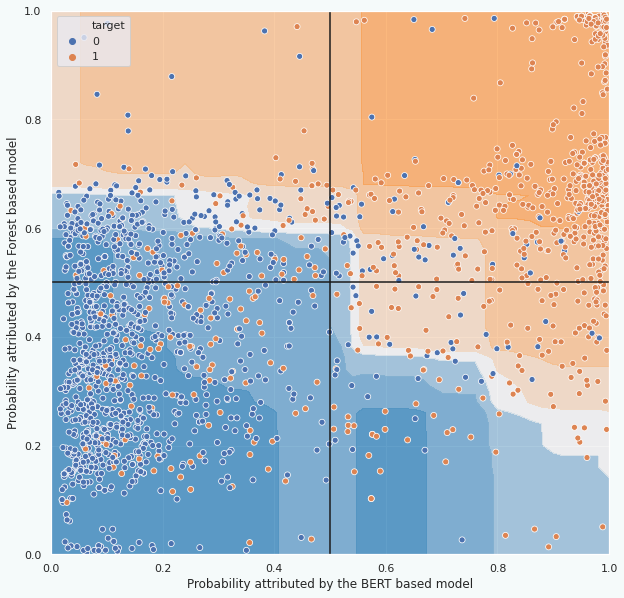
In the above figure we see that the final model mostly splits the space in two according to a line in the middle (the white part of the background). This split essentially preserves the prediction of the BERT-based model predicts. The performance should therefore be very similar to the performance of the BERT-based model. And when assessing the performance of the model we indeed get similar results as the BERT-based model:
Training scores:
precision=0.87 recall=0.81 f1=0.84
Validation scores:
precision=0.91 recall=0.75 f1=0.83
Integrate the whole model into a pipeline
A pipeline is a chain of processing steps for the data, the last step often being the machine learning model. When the last step is the machine learning model, we call this step the “estimator”. In our case, the estimator is a “classifier”, since the goal of the model is to classify things. When an estimator is not a classifier, it is in general a “regressor”. In particular, we include a series of steps called “transformers” before the model. They allow processing and preparing the data. The use of a series of transformers makes the code readable and less prone to errors. We have already seen an example of transformers in the feature extraction section. As I have explained in this section, transformers are useful to avoid label leakage that would make the model look better than it really is. Pipelines are a natural way of chaining these transformers and the model. Pipelines also simplify the deployment of the model.
The downside of using pipelines, is that they can make the model explanation more convoluted. That is one of the reasons why in this post I have separately talked about data preparation, the models, their explanations and interpretations, and only now about pipelines.

In the following I show the definition of some transformers for the BERT model, and then for the meta-data based model (which uses the Random Forest Classifier). Then, I show how to integrate these transformers into a pipeline to which I add the machine learning model itself (the classifier). Finally, I show how to combine the two pipelines into a single one with the stacking technique I have presented in a previous section. You will find all the details in my Jupyter Notebook.
Let me start by showing the definitions of some transformers. For example in Figure 9. you can see that the BERT based model is preceded by a Text Cleaner, which can be defined as follows.
# Define the Text Cleaner
def clean_text(X):
    X = pd.Series(X)
    X = X.copy()

    return X.apply(lambda s: clean(s))  # The function "clean" is the function we talked about in the begining of the post.

Cleaner_text = skl.preprocessing.FunctionTransformer(clean_text)  # This is the Text Cleaner transformer
In the meta-data based model I use a feature additioner transformer. This transformer adds features to the entry data frame as I explained in a previous section. This transformer is more involved than the previous text cleaner, so I need to create a subclass of the “base.TransformerMixin” class from scikit-learn.
# Transformer that will add features: "feature extraction"

class AddFeaturesTransformer(skl.base.BaseEstimator, skl.base.TransformerMixin):
    def __init__(self, column, ngram__n = 2, n_ngrams=100):
        super().__init__()
        self.n = ngram__n
        self.n_ngrams = n_ngrams
        self.mention_counter = CountMentionsInClass()
        self.ngram_counter = CountTopNGramsInClass(ngram__n, n_ngrams)
        self.column = column

    def fit(self, X, y, column = None):
        X = pd.DataFrame(X) ; X = X.copy()
        y = pd.Series(y) ; y = y.copy()

        if column is None:
            column=self.column

        if type(column) not in [int, str]:
            raise TypeError("{} is not int or str".format(type(column)))

        if type(column)==int:
            column = X.columns[column]

        self.mention_counter.fit(X, y, column=column)
        self.ngram_counter.fit(X, y, column=column)

        return self

    def transform(self, X, column=None):
        X = pd.DataFrame(X) ; X = X.copy()

        if column is None:
            column=self.column

        if type(column) not in [int, str]:
            raise TypeError("{} is not int or str".format(type(column)))

        if type(column)==int:
            column = X.columns[column]

        # count the number of hashtags
        X['hastags_count'] = X[column].map(lambda text: sum([char=='#' for char in text]) )
        # count all cap words
        X['capital_words_count'] = X[column].map( lambda text: sum( [word==word.upper() for word in text.split()] ) )
        # word_count
        X['word_count'] = X[column].apply(lambda x: len(str(x).split()))
        # unique_word_count
        X['unique_word_count'] = X[column].apply(lambda x: len(set(str(x).split())))
        # url_count
        X['url_count'] = X[column].apply(lambda x: len([w for w in str(x).lower().split() if 'http' in w or 'https' in w]))
        # mean_word_length
        X['mean_word_length'] = X[column].apply(lambda x: np.mean([len(w) for w in str(x).split()]))
        # char_count
        X['char_count'] = X[column].apply(lambda x: len(str(x)))
        # punctuation_count
        X['punctuation_count'] = X[column].apply(lambda x: len([c for c in str(x) if c in string.punctuation]))
        # mention_count
        X['mention_count'] = X[column].apply(lambda x: len([c for c in str(x) if c == '@']))
        # count mentions in target classes
        X = self.mention_counter.transform(X, column=column)
        # compute de difference between  mentions in disasters and mentions not in disasters
        X["difference_mentions_count"] = X["count_mentions_in_disaster"] - X["count_mentions_in_ndisaster"]
        # count ngrams in target classes
        X = self.ngram_counter.transform(X, column=column)
        # compute de difference between ngrams in disasters and mentions not in disasters
        X[f"difference_{self.n}-grams_count"] = X[f"count_{self.n}-grams_in_disaster"] - X[f"count_{self.n}-grams_in_ndisaster"]

        return X

    def fit_transform(self, X, y, column=None):

        if column is None:
            column=self.column

        return super().fit_transform(X, y, column=column)


Feature_additioner = AddFeaturesTransformer(column='text') # Here is the transformer
Once the relevant transformers are defined, we can group them into a pipeline, for example we can group three transformers as follows:
# Preprocessor pipeline
preprocessor = Pipeline([('nan_filler', Categorical_Nan_Filler),
                         ('cleaner_keywords', Cleaner_keywords),
                         ('feature_additioner', Feature_additioner)
                ])
Then, we can include this pipeline into another pipeline.
encode_scale = ColumnTransformer([('scaler',StandardScaler(), numerical_metaData_features),
                                  ('enc', OneHotEncoder(handle_unknown='ignore'), cat_metaData_features)]).fit(X_train,y_train)

# Here is the final meta-data based classifier. It will later be combined to the BERT based classifier.
metaData_clf = Pipeline([('preprocessor', preprocessor),
                         ('encode_scale', encode_scale),
                         ('rand_forest', RandomForestClassifier(max_depth=6, class_weight='balanced'))]
               )
The BERT pipeline is defined as follows (see also Figure 9.):
# Define the BERT model pipeline that takes a data frame as input

Bert_model = KerasClassifier(build_bert_model)

Cleaner_text = skl.preprocessing.FunctionTransformer(clean_text)


Bert_clf = Pipeline([('cleaner_text', Cleaner_text),
                     ('bert_model', Bert_model)
                    ])

Bert_clf_with_col_select = Pipeline([('column_selector', Column_selector),('bert_clf',Bert_clf)])
In the end we can group these two pipeline using the stacking technique. To do so, I have programmed my own stacking class (see code here). Then, in order to group the two pipelines I simply need the following:
# Define the final classifier

final_clf = MyStackingClassifier(estimators=[('Bert_clf', Bert_clf_with_col_select), ('rnd_forest', metaData_clf)],
                                final_estimator=RandomForestClassifier(max_depth=3, class_weight='balanced'))
This final model can be trained as a normal model even though internally a lot of things will happen:
final_clf.fit(X_train, y_train)
We can look at the final score of the model:
y_val_pred = final_clf.predict(X_val2)

# validation score
print("\nValidation scores:\n",
      "precision={:.2f}".format(skl.metrics.precision_score(y_true=y_val, y_pred=y_val_pred)),
      "recall={:.2f}".format(skl.metrics.recall_score(y_true=y_val, y_pred=y_val_pred)),
      "f1={:.2f}".format(skl.metrics.f1_score(y_true=y_val, y_pred=y_val_pred))
      )
Validation scores:
precision=0.87 recall=0.79 f1=0.83
The score is essentially the same as for the BERT model alone. As expected there was no improvement due to the combination of the models. Now, let us see what are the tweets the model got wrong:
# Look at the tweets where the model was wrong

indices = [i for i in range(len(y_val2)) if y_val_pred[i] != y_val2.iloc[i]]

end = 20

for tweet, idx in zip(X_val2['text'].loc[y_val_pred != y_val2].iloc[:end], indices):
    print(f'pred = {y_val_pred[idx]}', f'true = {y_val2.iloc[idx]}  ', tweet)
By running the above code we essentially get (up to formatting) the following:
| prediction | true | tweet |
|---|---|---|
| 0 | 1 | @todd_calfee so @mattburgener wanted to see that info on blight u got |
| 0 | 1 | I WAS PEACEFULLY SITTING IN MY ROOM AND I HEARD THIS LOUD BANG OF SOMETHING FALLING |
| 0 | 1 | TodayÛªs storm will pass; let tomorrowÛªs light greet you with a kiss. Bask in this loving warmth; let your soul return to bliss. |
| 0 | 1 | @TheHammers_ @tonycottee1986 alsowhat if some of the 1st team players got injured?Then Bilic would get slated for playing themhe can’t win |
| 0 | 1 | #hot Funtenna: hijacking computers to send data as sound waves [Black Hat 2015] http://t.co/J2aQs5loxu #prebreak #best |
| 1 | 0 | Haley Lu Richardson Fights for Water in The Last Survivors (Review) http://t.co/oObSCFOKtQ |
| 0 | 1 | My precious olive tree lost this battle…another crazy windstorm in #yyc! @weathernetwork http://t.co/N00DVXEga2 |
| 0 | 1 | I can probably skip on these basic life maintenance things for a few days. (cut to burning buildings people screaming in the streets) |
| 0 | 1 | US Navy Sidelines 3 Newest Subs - http://t.co/guvTIzyCHE: DefenseNews.comUS Navy Sidelines 3 Newest SubsD… http://t.co/SY2WhXT0K5 #navy |
| 1 | 0 | One thing you can be sure of. There will never be bush fires in Scotland as the ground is always soaking wet???? |
| 0 | 1 | @SophieWisey I couldn’t. #mudslide |
| 0 | 1 | Still rioting in a couple of hours left until I have to be up for class. |
| 0 | 1 | The Dress Memes Have Officially Exploded On The Internet http://t.co/3drSmxw3cr |
| 0 | 1 | Damn that sinkhole on sunset???? |
| 0 | 1 | 627% but if they had lower striked than 16 I would have gone even further OTM. This could really fall off a cliff. |
| 0 | 1 | Going back to Gainesville will be the death of me |
| 1 | 0 | #landslide while on a trip in #skardu https://t.co/nqNWkTRhsA |
| 0 | 1 | Imagine a room with walls that are lava lamps. |
| 0 | 1 | Is it seclusion when a class is evacuated and a child is left alone in the class to force compliance? #MoreVoices |
| 0 | 1 | You can never escape me. Bullets don’t harm me. Nothing harms me. But I know pain. I know pain. Sometimes I share it. With someone like you. |
We have here the 20 first tweets of the validation set where the model was “wrong” according to their target label. Let us have a look to the three first of them:
- For the first tweet it is hard to say without more context, but I personally think this should not be considered as a disastrous tweet. Still, the label of this tweet is \(1\) which means that whoever made the data set considered that this tweet was talking about a disaster.
- The second tweet talk about a loud noise of some object falling on the floor. Without more context this does not sound like a disaster, but once again it is labeled as a disaster for some reason.
- The third looks like the lyrics of a song, which again, despite the presence of the word “storm”, should not be classified as a disaster but is labeled as such.
I’ll let you make your own opinion on the other examples, but it seems to me that for the majority of them, the labeling is either wrong or the tweet is sufficiently vague and context dependent so that it could be both about a disaster or not. This leads me to think that there is a substantial fraction of the tweets that have been mislabeled. Note that this mislabeling not only affects the evaluation of the model, but also its training. If the fraction of mislabeled tweets is sufficiently high this might prevent any model to get a better score than some limit score. To remedy this problem, one would need to go through the whole data set to relabel the tweets properly.
Conclusion
Let me summarize all we have seen in this post. First, I have presented the data set, and how to clean it thanks to the vocabulary coverage with respect to existing vocabulary list. I then showed that we can extract from the tweets some special features that can be of interest. I then showed two simple models that use these newly created features to classify the tweets. I explained what was features importance and that it can be used to select the best features among the ones I created. Not only that, but I went a bit further in the explanation of the model thanks to the shap library. This further allows to check that the model makes sense, and understand why the model performs the classification the way it does. Then, I showed how to use the pretrained BERT model to classify the tweets directly without passing through features added by hand: The features are automitacally extracted by the BERT layer. We then saw that even such a complicated model can be interpreted. In the end I showed that we can combine different models into a single one using the stacking technique. Finally, I showed how to wrap everything into a pipeline.
Is this all we can do in such a project? You might have already guessed that the answer is no. In fact, it depends on whether you are satisfied with the results of the model. In this post I only presented several of the important steps of such a project. The goal being to present a broad scope of the tools that can be used and the big steps we take in a text classification project. But I did not explore in details the way of improving the model once we reached this point. And as you can see the model gets a score of about \(83\%\), which depending on the application might or might not be enough.
Let me briefly tell you some possible ways one can further improve the model. First, since the feature I added are all implicitly present in the text, I would remove the meta-data based model and use only the BERT based model, unless you want to add information about the context of the tweets. Then I would try to see why the misclassified tweet are misclassified by looking at the text explainer. Also, we have seen that several of the tweets where the model makes mistakes are either quite ambiguous or they have been mislabeled. This mislabelling affects both the training and the evaluation. So carefully relabelling the data set is a step that can help even though it’s a tedious work. One other tedious work could be to clean even more the tweets and maybe remove stop words which is something I have not done. Another step that can indirectly improve the model is to try and use different versions of BERT. There are versions that are lighter than others. Even though this is not likely to improve the accuracy of the model it will make it run and train faster.
In the future, I plan to modify this model, and train it on a different set of data, in order to write a small app that can classify tweets into one of three categories: constructive comment, neutral and insult/offensive. This will be the topic of a future post.
References
[RSG] Ribeiro, Marco Tulio, Sameer Singh, and Carlos Guestrin. “” Why should I trust you?” Explaining the predictions of any classifier.” Proceedings of the 22nd ACM SIGKDD international conference on knowledge discovery and data mining. 2016.
-
Note that I removed the location column from the data set. This is because there are too many unique locations, which makes this column not useful for the classification. ↩
-
This step is not necessary for a tree based model like the Random Forest since they are not sensitive to scaling, but it is a good habit to get, so I choose to do it anyways. In all cases, I’ll have to do that for the Logistic Regression in the next section. ↩
